Templates for Data Structures and Algorithms
Contents
| Symbol | Designation |
|---|---|
| ✓ | This is a problem from LeetCode's interview crash course. |
| ✠ | This is a problem stemming from work done through Interviewing IO. |
| ★ | A right-aligned ★ (one or more) indicates my own personal designation as to the problem's relevance, importance, priority in review, etc. |
- Backtracking
- Binary search
- Dynamic programming
- Graphs
- Greedy algorithms
- Heaps
- Linked lists
- Matrices
- Sliding window
- Stacks and queues
- Trees
- Manually determine order of nodes visited ("tick trick")
- Pre-order traversal
- Post-order traversal
- In-order traversal
- Level-order traversal
- Level-order (BFS)
- Induction (solve subtrees recursively, aggregate results at root)
- Traverse-and-accumulate (visit nodes and accumulate information in nonlocal variables)
- Combining templates: induction and traverse-and-accumulate
- Two pointers
- Miscellaneous
Backtracking
Remarks
TBD
def fn(curr, OTHER_ARGUMENTS...):
if (BASE_CASE):
# modify the answer
return
ans = 0
for (ITERATE_OVER_INPUT):
# modify the current state
ans += fn(curr, OTHER_ARGUMENTS...)
# undo the modification of the current state
return ans
Examples
LC 46. Permutations (✓) ★★
Given an array nums of distinct integers, return all the possible permutations. You can return the answer in any order.
class Solution:
def permute(self, nums: List[int]) -> List[List[int]]:
def backtrack(curr):
if len(curr) == len(nums):
permutations.append(curr[:]) # note that we append a _copy_ of curr
return
for num in nums:
if num not in curr:
curr.append(num)
backtrack(curr)
curr.pop()
permutations = []
backtrack([])
return permutations
What actually is a permutation of nums? It's essentially all possible orderings of the elements of nums such that no element is duplicated. A backtracking strategy to generate all permutations sounds promising — what would the base case be? It would be when the current permutation being generated, say curr, has the same length as the input array nums: curr.length == nums.length (of course, this assumes we've done our due diligence and have prevented duplicates from being added to curr). The base case of curr.length == nums.length means we have completed the process of generating a permutation and we cannot go any further; specifically, if we look at the process of generating permutations as a tree, then completing the generation of a permutation means we have reached a leaf node, as illustrated in the following image for the input nums = [1, 2, 3]:
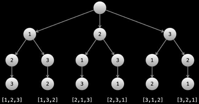
Building all permutations for this problem, where the input is an array of numbers, means we need all elements to make an appearance at the first index, all other elements to make an appearance at the second index, and so on. Hence, we should loop over all elements of nums for each call to our backtrack function, where we should always check to see if a number is already in curr before adding it to curr. Each call to backtrack is like visiting a node in the tree of candidates being generated. The leaves are the base cases/answers to the problem.
For the solution given above, if we simply add print(curr) after the line curr.append(num), then we can very clearly see how each call to backtrack is like visiting a node in the tree (it's like performing a DFS on an imaginary tree):
[1]
[1, 2]
[1, 2, 3] # complete permutation (leaf node)
[1, 3]
[1, 3, 2] # complete permutation (leaf node)
[2]
[2, 1]
[2, 1, 3] # complete permutation (leaf node)
[2, 3]
[2, 3, 1] # complete permutation (leaf node)
[3]
[3, 1]
[3, 1, 2] # complete permutation (leaf node)
[3, 2]
[3, 2, 1] # complete permutation (leaf node)
The entire list of complete permutations is then returned as the answer:
[[1, 2, 3], [1, 3, 2], [2, 1, 3], [2, 3, 1], [3, 1, 2], [3, 2, 1]]
The time complexity above effectively amounts to roughly , because we iterate through all of nums for each call to backtrack, and membership to curr is a linear cost when curr is an array, and then we're guaranteed to make calls to backtrack, and each call to backtrack then results in calls, and so forth. If we wanted to make a micro-optimization, then we could introduce a hash set to make the membership checks on curr instead of , but this change pales in comparison to the factorial cost of calling backtrack so many times:
class Solution:
def permute(self, nums: List[int]) -> List[List[int]]:
def backtrack(curr):
if len(curr) == len(nums):
permutations.append(curr[:])
return
for num in nums:
if num not in lookup:
curr.append(num)
lookup.add(num)
backtrack(curr)
curr.pop()
lookup.remove(num)
lookup = set()
permutations = []
backtrack([])
return permutations
LC 78. Subsets (✓) ★★
Given an integer array nums of unique elements, return all possible subsets (the power set). The solution set must not contain duplicate subsets. Return the solution in any order.
class Solution:
def subsets(self, nums: List[int]) -> List[List[int]]:
def backtrack(curr, num_idx):
subs.append(curr[:])
if num_idx == len(nums): # note that this base case is implied
return # since `backtrack` is only called in the
# for loop when `num_idx < len(nums)`
for i in range(num_idx, len(nums)):
curr.append(nums[i])
backtrack(curr, i + 1)
curr.pop()
subs = []
backtrack([], 0)
return subs
This problem is quite similar to LC 46. Permutations but with some very notable differences, namely container length and element order:
- Length: A subset can have any length from
0throughn(wherenis the size of the input array of distinct integers), inclusive, but a permutation has a fixed length ofn. - Order: The containers
[1, 2, 3]and[3, 2, 1]are considered to be different permutations but the same subset.
If we have a problem where containers like those above are considered to be duplicates and we do not want to consider duplicates (e.g., such as this problem concerned with finding subsets), then a common "trick" is to add a rule where each call of the backtrack function allows us to only consider elements that come after the previously processed element:
This is a very common method of avoiding duplicates in backtracking problems — have an integer argument that represents a starting point for iteration at each function call.
For example, in this problem, we start with the root being the empty container, []:
[]
With nums = [1, 2, 3], we can clearly consider each element as the beginning of its own subset:
[ ]
/ | \
[1] [2] [3]
Now what? Remember that calling backtrack is like moving to another node; hence, to respect the strategy remarked on above, when we move to another node, that node should only involve elements that come after the one we have just processed. This means the tree of possibilities above should end up looking like the following:
[ ] # level subsets: []
/ | \
[1] [2] [3] # level subsets: [1], [2], [3]
/ \ |
[2] [3] [3] # level subsets: [1,2], [1,3], [2,3]
|
[3] # level subsets: [1,2,3]
The actual order of subset generation from our solution code is not hard to anticipate in light of the strategy we've been discussing, where, again, we're basically doing a DFS on an imaginary tree, and once we hit the last indexed element (i.e., when index == len(nums)) we move back up the tree from child to parent:
[
[],
[1],
[1,2],
[1,2,3],
[1,3],
[2]
[2,3]
[3]
]
The order conjectured above is confirmed by the return value of our solution when nums = [1, 2, 3]:
[[], [1], [1, 2], [1, 2, 3], [1, 3], [2], [2, 3], [3]]
The process becomes even clearer if we add the print statement print(subs) after subs.append(curr[:]) as well as the print statement print('COMPLETED') after if num_idx == len(nums):. Making these modifications and running the solution code again on the input nums = [1,2,3] results in the following being printed to standard output:
[[]]
[[], [1]]
[[], [1], [1, 2]]
[[], [1], [1, 2], [1, 2, 3]]
COMPLETED
[[], [1], [1, 2], [1, 2, 3], [1, 3]]
COMPLETED
[[], [1], [1, 2], [1, 2, 3], [1, 3], [2]]
[[], [1], [1, 2], [1, 2, 3], [1, 3], [2], [2, 3]]
COMPLETED
[[], [1], [1, 2], [1, 2, 3], [1, 3], [2], [2, 3], [3]]
COMPLETED
[[], [1], [1, 2], [1, 2, 3], [1, 3], [2], [2, 3], [3]]
Note that the text 'COMPLETED' is only ever printed after an element/subset has been added to subs that ends with 3, which corresponds to the leaves of the tree shown earlier.
To summarize, when generating permutations, we had a length requirement, where we needed to use all of the elements in the input; hence, we only considered leaf nodes as part of the actual returned answer. With subsets, however, there is no length requirement; thus, every node should be in the returned answer, including the root node, which is why the very first line of the backtrack function is to add a copy of curr to the returned answer subs.
LC 77. Combinations (✓) ★★
Given two integers n and k, return all possible combinations of k numbers out of 1 ... n. You may return the answer in any order.
class Solution:
def combine(self, n: int, k: int) -> List[List[int]]:
def backtrack(curr, start_val):
if len(curr) == k:
combinations.append(curr[:])
return
for i in range(start_val, n + 1):
curr.append(i)
backtrack(curr, i + 1)
curr.pop()
combinations = []
backtrack([], 1)
return combinations
It can be very helpful to sketch out a tree of possibilities if we suspect backtracking may be an effective strategy for coming up with a solution (just like sketching out things for general tree problems, linked list problems, etc.).
The root of our tree would be [], the empty list. Unlike in LC 78. Subsets, there is an explicit length requirement in terms of the elements that can be added to the container we must ultimately return; hence, not all nodes in the tree of possibilities will represent entities that should be added to our answer array.
What is clear is that each entry added to the list we must return must have a length of k, and it must contain numbers from the list [1, ..., n], inclusive, where no number in the k-length list is duplicated. This means we should consider combining some of the strategy points we used in both LC 46. Permutations and LC 78. Subsets, namely using a length requirement as part of the base case as well as preventing duplicates from being considered, respectively.
The thinking goes something like the following: start with the empty list, [], as the root of the tree:
[]
Each k-length list can have a number from [1, ..., n], inclusive; thus, the root should have n children, namely nodes with values from 1 through n (the example below uses the values of n = 4, k = 2 from the first example on LeetCode):
[ ]
[1] [2] [3] [4]
Now what? A complete solution will be generated only when the path has length k, but each path right now has a length of 1 (but k = 2 for this example). To keep generating paths (i.e., possible solutions), we need to avoid considering duplicates, which means for each node value i, we only subsequently consider node values [i + 1, ..., n], which results in our overall tree looking like the following:
[ ]
[1] [2] [3] [4]
[2] [3] [4] [3] [4] [4]
Since the input specifies k = 2, the tree above suffices to report the following as the combinations list:
[
[1,2],
[1,3],
[1,4],
[2,3],
[2,4],
[3,4]
]
LC 797. All Paths From Source to Target (✓) ★
Given a directed acyclic graph (DAG) of n nodes labeled from 0 to n - 1, find all possible paths from node 0 to node n - 1, and return them in any order.
The graph is given as follows: graph[i] is a list of all nodes you can visit from node i (i.e., there is a directed edge from node i to node graph[i][j]).
class Solution:
def allPathsSourceTarget(self, graph: List[List[int]]) -> List[List[int]]:
def backtrack(curr_path, node):
if node == len(graph) - 1:
paths.append(curr_path[:])
return
for neighbor in graph[node]:
curr_path.append(neighbor)
backtrack(curr_path, neighbor)
curr_path.pop()
paths = []
backtrack([0], 0)
return paths
This is a great backtracking problem because backtracking is not necessarily the obvious first strategy of attack. Even if we do think of backtracking, how exactly should we proceed? This becomes much clearer (again!) once we start to sketch out the tree of possibilities. What would the root of our tree be? It has to be node 0 since our goal is to find all paths from node 0 to node n - 1. This also suggests something about our base case: we should terminate path generation whenever node n - 1 is reached. We don't have to worry about cycles or anything like that since we're told the graph is a DAG. Additionally, the graph is already provided as an adjacency list which makes traversing each node's neighbors quite easy.
So what's the strategy? Let's start with our root node (which needs to be part of every solution):
0
Now what? Each neighbor of node 0 needs to be considered (we're trying to get to node n - 1 from node 0 in whatever way is possible, which means exploring all possible paths). Let's use the input of the second example on LeetCode for a concrete illustration: graph = [[4,3,1],[3,2,4],[3],[4],[]]. This graphs looks like the following:
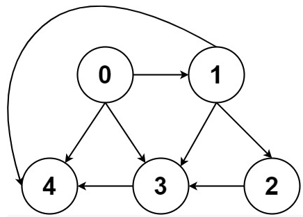
As stated above, from 0 we need to consider each of its neighbors:
0
/ | \
1 3 4
The tree above makes it clear [0,4] will be one possible path, but what are the other possible paths? It looks like leaf nodes will be the complete solutions that need to be added to our answer that we ultimately return. For each node that is not 4 (i.e., n - 1 == 4 in this case), we need to consider each possible neighbor (this will not be endless because we're told the graph is a DAG). Considering the neighbors for each node means our tree of possibilities ultimately ends up looking as follows:
0
/ | \
1 3 4
/ | \ |
2 3 4 4
| |
3 4
|
4
Hence, the set of possible paths is as expected:
[[0,4],[0,3,4],[0,1,3,4],[0,1,2,3,4],[0,1,4]]
LC 17. Letter Combinations of a Phone Number (✓) ★★
Given a string containing digits from 2-9 inclusive, return all possible letter combinations that the number could represent. Return the answer in any order.
A mapping of digit to letters (just like on the telephone buttons) is given below. Note that 1 does not map to any letters.

class Solution:
def letterCombinations(self, digits: str) -> List[str]:
if not digits:
return []
keypad = {
'2': 'abc',
'3': 'def',
'4': 'ghi',
'5': 'jkl',
'6': 'mno',
'7': 'pqrs',
'8': 'tuv',
'9': 'wxyz'
}
def backtrack(curr, start_idx):
if len(curr) == len(digits):
combinations.append("".join(curr))
return
for i in range(start_idx, len(digits)):
digit = digits[i]
for letter in keypad[digit]:
curr.append(letter)
backtrack(curr, i + 1)
curr.pop()
combinations = []
backtrack([], 0)
return combinations
As with most other backtracking problems, it helps if we start by sketching out the tree of possibilities, where we can imagine the root being an empty string:
''
Now let's consider the input digits = "23", the input for the first example on LeetCode. The desired output is ["ad","ae","af","bd","be","bf","cd","ce","cf"]. How can this be achieved? The first digit is 2, which means 'a', 'b', and 'c' are valid starting letters for combinations:
' '
/ | \
'a' 'b' 'c'
We do not want to add duplicates of these letters for subsequent possible combinations but instead consider the potential letters arising from the next digit (i.e., we want to prevent processing duplicates by only ever processing digits after the current digit). The next digit in this case is 3 which corresponds to possible letters 'd', 'e', and 'f'. Our tree now looks like the following:
' '
/ | \
'a' 'b' 'c'
/ | \ / | \ / | \
'd' 'e' 'f' 'd' 'e' 'f' 'd' 'e' 'f'
The tree of possibilities above makes it clear the letter combinations we should return are as follows, as expected:
[
'ad',
'ae',
'af',
'bd',
'be',
'bf',
'cd',
'ce',
'cf',
]
LC 39. Combination Sum (✓) ★
Given an array of distinct integers candidates and a target integer target, return a list of all unique combinations of candidates where the chosen numbers sum to target. You may return the combinations in any order.
The same number may be chosen from candidates an unlimited number of times. Two combinations are unique if the frequency of at least one of the chosen numbers is different.
It is guaranteed that the number of unique combinations that sum up to target is less than 150 combinations for the given input.
class Solution:
def combinationSum(self, candidates: List[int], target: int) -> List[List[int]]:
def backtrack(path, path_sum, next_path_node_idx):
if path_sum == target:
paths.append(path[:])
return
for i in range(next_path_node_idx, len(candidates)):
candidate = candidates[i]
if path_sum + candidate <= target:
path.append(candidate)
backtrack(path, path_sum + candidate, i)
path.pop()
paths = []
backtrack([], 0, 0)
return paths
This problem is similar to LC 77. Combinations, but now we are taksed with generating all combinations of candidates such that each candidate number is allowed however many times we want, but the sum of the numbers for each combination/mixture of candidates has to equal the given target.
Start by drawing a tree!
[]
Each number in candidates may be part of a path sum we want to return, where the sum of the elements in the path equates to target. Let's use the input provided in the first example on LeetCode: candidates = [2,3,6,7], target = 7:
[ ]
/ / \ \
2 3 6 7
The problem description indicates any number may be reused however many times we desire, but we still don't want to generate duplicates such as [2,2,3], [2,3,2], etc. How can we avoid doing this? We can use the same strategy that many other backtracking problems use (i.e., ensure we only begin processing elements that are either the current element itself or elements that come after the current element):
[ ]
/ / \ \
2 3 6 7
/ / \ \ /|\ / \ |
2 3 6 7 3 6 7 6 7 7
..................................
When do we stop the process of generating paths? Since all possible values in candidates are positive, this necessarily means a path is no longer valid if its path sum exceeds the given target value.
Note that the following lines in the solution above are important:
# ...
for i in range(next_path_node_idx, len(candidates)):
candidate = candidates[i]
if path_sum + candidate <= target:
path.append(candidate)
# ...
It might be tempting to modify path_sum with the candidate value before entering the if block, but this would be a mistake. Why? Because the list of candidates is not necessarily ordered; hence, if we made the update path_sum += candidate and the new path_sum exceeded target, then we would no longer consider that path, but this would also prevent us from exploring other branches using candidates of a possibly lesser value where path_sum + candidate did not exceed target.
LC 79. Word Search (✓) ★★★
Given an m x n board and a word, find if the word exists in the grid.
The word can be constructed from letters of sequentially adjacent cells, where "adjacent" cells are horizontally or vertically neighboring. The same letter cell may not be used more than once.
class Solution:
def exist(self, board: List[List[str]], word: str) -> bool:
def valid(row, col):
return 0 <= row < m and 0 <= col < n
def backtrack(row, col, word_idx, seen):
if word_idx == len(word):
return True
for dr, dc in dirs:
next_row, next_col = row + dr, col + dc
if valid(next_row, next_col) and (next_row, next_col) not in seen:
next_char = board[next_row][next_col]
if next_char == word[word_idx]:
seen.add((next_row, next_col))
if backtrack(next_row, next_col, word_idx + 1, seen):
return True
seen.remove((next_row, next_col))
return False
m = len(board)
n = len(board[0])
dirs = [(1,0),(-1,0),(0,1),(0,-1)]
for row in range(m):
for col in range(n):
if board[row][col] == word[0] and backtrack(row, col, 1, {(row, col)}):
return True
return False
This problem has a very DFS feel to it, but what makes this a backtracking problem and not a strict DFS problem is because we may visit a square multiple times on the same initial function call. For example, suppose we're looking for the word CAMERA in the following grid:
CAM
ARE
MPS
We may start exploring as follows (each | represents the path taken):
C A M
|
A R E
|
M P S
The M-letter above does not have E as a neighbor so we remove the M from consideration and move back up to A, which also does not have an M-neighbor except the one we just visited, which we know leads to nothing. So we remove A as well and we're back at C, and we note C does have another A-neighbor it can visit. And we end up seeing the following as a valid path:
C -> A -> M
|
A <- R <- E
M P S
This path visits the A under C again in order to come up with a valid path. Thus, while we may not be allowed to use a square more than once for the answer, there are possibly multiple ways to use a square to form different candidates, as illustrated above.
We should still use a set seen like we would normally do with DFS solutions so as to avoid using the same letter in the same path. Unlike in DFS solutions, however, we will remove from the set seen when backtracking and it's been determined that a path solution is no longer possible — we should only ever traverse an edge in the graph if we know that the resultant path could lead to an answer. Thus, we can also pass an index variable word_idx that indicates we are currently looking for word[word_idx], and then only move to (next_row, next_col) if word[word_idx] is the correct letter.
Since the answer could start from any square whose letter matches word[0], we need to systematically start our backtracking approach from any square with word[0] as its letter. If we exhaust all such squares and never find word, then we should return false. Of course, if we do find word in the midst of one of our backtracking approaches, then we return true immediately.
LC 52. N-Queens II (✓) ★★★
The n-queens puzzle is the problem of placing n queens on an n x n chessboard such that no two queens attack each other.
Given an integer n, return the number of distinct solutions to the n-queens puzzle.
class Solution:
def totalNQueens(self, n: int) -> int:
def backtrack(row, cols, diagonals, anti_diagonals):
# base case: n queens have been placed
if row == n:
return 1
solution = 0
for col in range(n):
diagonal = row - col
anti_diagonal = row + col
# queen is not placeable, move to considering next column
if (col in cols or diagonal in diagonals or anti_diagonal in anti_diagonals):
continue
# add the queen to the board
cols.add(col)
diagonals.add(diagonal)
anti_diagonals.add(anti_diagonal)
# move to next row with the updated board state
solution += backtrack(row + 1, cols, diagonals, anti_diagonals)
# remove the queen from the board since we have
# explored all valid paths using the above backtrack function call
cols.remove(col)
diagonals.remove(diagonal)
anti_diagonals.remove(anti_diagonal)
return solution
return backtrack(0, set(), set(), set())
This problem is difficult. And it's often used to explain backtracking at various learning levels (e.g., university and college classes). The solution to this problem is informative, especially in regards to how we might want to go about modeling backtracking solutions to other problems.
Whenver we make a call to backtrack, we're doing so by describing the state of whatever it is that is important for consideration in solving the problem at hand. For some problems, maybe that state involves a string and the number of used left and right parentheses (e.g., LC 22. Generate Parentheses), maybe the state involves the row and column of a grid under consideration along with the cells already seen and the index of a word that represents a character for which we are searching (e.g., LC 79. Word Search). And maybe, as in this problem, the state needs to involve a chessboard!
What state should we consider tracking? We need to somehow keep track of rows and columns in some way. The trickier part about this problem involves the diagonals. Even though we have a board in this problem, this is not like a graph problem where we need to conduct a DFS or BFS — fundamentally, our job at each step is to place a queen on the board so that it is not under attack. This is the backtracking part where we narrow down the range of possibilities we consider — the brute force approach would involve generating all board possibilities with queens and then narrow down which solutions actually work, but that would involve placing queens on the board in positions that are being attacked, which means the rest of the generation of possibilities is useless. We want to place queens in positions where they are not being attacked and where whatever subsequent positions we consider can actually lead to a solution. Only once we find a solution do we start to undo queen placement and try other queen placements, but the key is that every placement must be one that could potentially lead to success.
With everything in mind above, how should we proceed? First, it's helpful to just think about how queens move on a chessboard: unlimited moves vertically, horizontally, diagonally (top left to bottom right), and anti-diagonally (top right to bottom left). If we are given n queens on an n x n chessboard, then it's clear that, at the end of the board configuration, each row must have a queen and each column must have a queen. The trickiest part is managing the diagonals effectively.
But we can start by working with the insight above about rows and columns. Each time backtrack is called should result in the placement of a queen on a new row; that is, we'll pass row as an argument to backtrack, and when we have finally reached row == n (i.e., rows 0 through n - 1 have been filled with queens), then we will know we have found a valid solution. Finding a workable position on any given row means processing all column positions on that row until we have found a position that is not under attack.
What about columns? As noted above, for each row being processed, we will iterate through all row positions (i.e., across all columns) until we find a column position that is not under attack. The row we are processing is definitely not under attack due to how we're processing rows, but how do we know whether or not each column is under attack? If another queen is on any column we're considering for a current row, then that column position is invalid because that other queen's line of attack runs through the current position we're considering. We need to consider the next column position. To keep track of which columns are already occupied by queens (i.e., which columns would be considered to be under attack when we're trying to add a new queen), whenever we add a queen to the board, we should add the column position of the queen to a set cols that we can use when we're trying to add subsequent queens.
Cool! We consider rows sequentially so it's guaranteed each row we're considering is not under attack. We have a set cols that shows which columns are occupied. It seems like we need a similar "strategy" for diagonals and anti-diagonals that we currently have for columns; that is, whenever we add a queen to the board, we should also note which diagonal and anti-diagonal just became occupied. But how do we effectively apply a singular label or marker to a diagonal or anti-diagonal that spans multiple positions on the board?
This seems really tricky to do at first until we make note of a brilliant observation concerning diagonal and anti-diagonal movement (R and C below represent row and column position, respectively):
-
diagonal movement (top left to bottom right): If we start at any cell
(R, C)and move one position up, then we will be at cell(R - 1, C - 1). If we move one position down, then we will be at(R + 1, C + 1). In general, if we letdranddcrepresent the change in row or column value, respectively, then we will find ourselves always moving from cell(R, C)to(R + dr, C + dc)on a given diagonal. Importantly, note thatdr == dcsince a change in any direction effects each value in the same way (e.g., moving 4 spaces up meansdr == dc == -4since the row and column values both decrease by 4).But how does any of this help in service of creating a unique label for a diagonal? The insight lies in how the row and column values relate to each other. Let
(R, C)be the coordinates of a cell on a diagonal, and let's label the cell as having valueR - C. Then what happens whenever we move from cell(R, C)to cell(R + dr, C + dc)? Sincedr == dc, we have(R + dr) - (C + dc) = R + dr - C - dr = R - C; that is, the label for any cell on a diagonal is the same: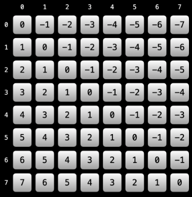
Hence, we should label visited diagonals by adding
row - colvalues to adiagonalsset. -
anti-diagonal movement (top right to bottom left): We can make a similar argument to the one above about effectively labeling anti-diagonals. Let
(R, C)represent any given cell on an anti-diagonal. Then moving up a cell would take us to cell(R - 1, C + 1)while moving down a cell would take us to cell(R + 1, C - 1); that is, the row and column values of a cell change at the same rate in an inversely proportional manner. We essentially havedr == dcagain, but there needs to be a sign difference in how we represent a movement from(R, C)to another cell:(R + dr, C - dc). Then(R + dr) + (C - dc) = R + dr + C - dr = R + C: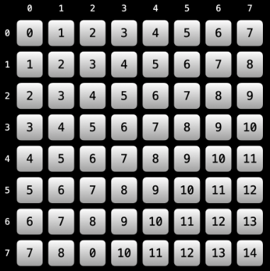
Hence, we should label visited anti-diagonals by adding
row + colvalues to ananti-diagonalsset.
LC 22. Generate Parentheses (✓) ★★★
Given n pairs of parentheses, write a function to generate all combinations of well-formed parentheses.
class Solution:
def generateParenthesis(self, n: int) -> List[str]:
def backtrack(curr_str, left_count, right_count):
if len(curr_str) == 2 * n:
valid_parens.append("".join(curr_str))
return
if left_count < n:
curr_str.append('(')
backtrack(curr_str, left_count + 1, right_count)
curr_str.pop()
if left_count > right_count:
curr_str.append(')')
backtrack(curr_str, left_count, right_count + 1)
curr_str.pop()
valid_parens = []
backtrack([], 0, 0)
return valid_parens
The editorial for this solution on LeetCode is quite good. The key insights (with the first being somewhat minor but the second one being critical):
- We should append the string we're building whenever its length is
2nbecause the string we're building, when taking a backtracking approach anyway, must have the potential to be valid and a complete solution at every point. Hence, once/if the candidate string reaches a length of2n, then we know the string satisfies the constraints of the problem and is a complete solution. - As a starting point, we can add as many left-parentheses as we want without fear of producing an invalid string (so long as the number of left parentheses we add doesn't exceed
n). We then need to start adding right parentheses. But how can we add right parentheses in general? We should only ever consider adding a right parenthesis when the total number of left parentheses exceeds the number of right parentheses. That way when we add a right parenthesis there's a chance the subsequent string could be a well-formed parenthetical string of length2n, as desired.
The LeetCode editorial linked above shows how sketching out a tree of possibilities is very useful for this problem, where the following illustration is for the beginning of the case where n = 2:
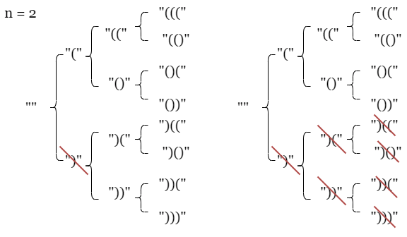
We can start to see how the logic of the solution above makes sense. For the sake of completeness and concreteness, consider the input of the first example on LeetCode, n = 3, and the corresponding desired output:
["((()))","(()())","(())()","()(())","()()()"]
We can make our own diagram that shows how each solution is built (the x indicates that potential solution path is longer pursued since further work on that path cannot possibly lead to a correct answer):
_____________________________________________________"
/ \
_________________________________________________(________________________________________________ x
/ \
_______________________((_______________________ _______________________()
/ \ / \
(((___ _________________(()________________ _________________()(________________ x
/ \ / \ / \
x ((()____ (()(____ _________(()) ()((____ _________()()
/ \ / \ / \ / \ / \
x ((())__ x (()()__ (())(__ x x ()(()__ ()()(__ x
/ \ / \ / \ / \ / \
x ((())) x (()()) x (())() x ()(()) x ()()()
As a note of reference, the tree above was generated using the binarytree package:
from binarytree import build2
my_tree = build2([
'"',
"(", 'x',
"((", "()", None, None,
"(((", "(()", "()(", "x",
"x", "((()", "(()(", "(())", "()((", "()()", None, None,
None, None, "x", "((())", "x", "(()()", "(())(", "x", "x", "()(()", "()()(", "x",
None, None, "x", "((()))", None, None, "x", "(()())", "x", "(())()", None, None, None, None, "x", "()(())", "x", "()()()"
])
root = my_tree.levelorder[0]
print(root)
LC 967. Numbers With Same Consecutive Differences (✓) ★★
Return all non-negative integers of length n such that the absolute difference between every two consecutive digits is k.
Note that every number in the answer must not have leading zeros. For example, 01 has one leading zero and is invalid.
You may return the answer in any order.
class Solution:
def numsSameConsecDiff(self, n: int, k: int) -> List[int]:
def digits_to_int(digits):
ans = digits[0]
for i in range(1, len(digits)):
ans = (ans * 10) + digits[i]
return ans
def backtrack(digit_arr):
if len(digit_arr) == n:
res.append(digits_to_int(digit_arr))
return
for num in range(10):
if abs(digit_arr[-1] - num) == k:
digit_arr.append(num)
backtrack(digit_arr)
digit_arr.pop()
res = []
for start_digit in range(1, 10):
backtrack([start_digit])
return res
The impossibility of leading zeros can complicate things if we're not careful. We still need to consider the digit 0 as part of potential constraint-satisfying integers. An easy way to handle this is to completely prevent 0 from being a possible leading digit at the outset. Execute the backtrack function for digit arrays that begin with each number 1 through 9, inclusive, and append complete solutions to an overall results array, res, that we ultimately return. It's easiest to manage the digits if we build each integer using a digits array and then return the actual integer once the digits array represents a constraint-satisfying integer.
LC 216. Combination Sum III (✓) ★
Find all valid combinations of k numbers that sum up to n such that the following conditions are true:
- Only numbers
1through9are used. - Each number is used at most once.
Return a list of all possible valid combinations. The list must not contain the same combination twice, and the combinations may be returned in any order.
class Solution:
def combinationSum3(self, k: int, n: int) -> List[List[int]]:
def backtrack(nums_arr, curr_sum, next_num):
if len(nums_arr) == k and curr_sum == n:
res.append(nums_arr[:])
return
for num in range(next_num, 10):
if curr_sum + num <= n:
nums_arr.append(num)
backtrack(nums_arr, curr_sum + num, num + 1)
nums_arr.pop()
res = []
backtrack([], 0, 1)
return res
The valid combinations can only involve positive integers, which means the sum we're building can only get bigger. Hence, we should only consider as possibilities combinations of integers for which the sum does not exceed n. Also, the numbers used as part of the combination need to be unique. Which means whenever we start with a certain number we should only ever consider subsequent integer values.
Binary search
Array
Remarks
TBD
def binary_search(arr, target):
left = 0 # starting index of search range (inclusive)
right = len(arr) - 1 # ending index of search range (inclusive)
result = -1 # result of -1 indicates target has not been found yet
while left <= right: # continue search while range is valid
mid = left + (right - left) // 2 # prevent potential overflow
if arr[mid] < target: # target is in right half
left = mid + 1 # (move `left` to narrow search range to right half)
elif arr[mid] > target: # target is in left half
right = mid - 1 # (move `right` to narrow search range to left half)
else: # target found (i.e., arr[mid] == target)
result = mid # store index where target is found (early return, if desired)
right = mid - 1 # uncomment to find first occurrence by narrowing search range to left half
# left = mid + 1 # uncomment to find last occurrence by narrowing search range to right half
if result != -1:
return result # target was found; return its index
else:
return left # target was not found; return insertion point to maintain sorted order
# NOTES:
# only one of the following lines should be uncommented in the else clause: `right = mid - 1` and `left = mid + 1` should
# `right = mid - 1` uncommented and `left = mid + 1` commented out results in searching for first occurrence of target
# `left = mid + 1` uncommented and `right = mid - 1` commented out results in searching for last occurrence of target
Examples
LC 704. Binary Search
Given an array of integers nums which is sorted in ascending order, and an integer target, write a function to search target in nums. If target exists, then return its index. Otherwise, return -1.
class Solution:
def search(self, nums: List[int], target: int) -> int:
left = 0
right = len(nums) - 1
while left <= right:
mid = left + (right - left) // 2
if target < nums[mid]: # target in left half, move right boundary
right = mid - 1
elif target > nums[mid]: # target in right half, move left boundary
left = mid + 1
else:
return mid # target at current mid position, return
return -1
The code above is the template for a basic binary search. We're guaranteed that the numbers in nums are unique, which means target, if it exists, will be found and the first index at which it occurs (and only index) will be returned.
LC 74. Search a 2D Matrix
Write an efficient algorithm that searches for a value in an m x n matrix. This matrix has the following properties:
- Integers in each row are sorted from left to right.
- The first integer of each row is greater than the last integer of the previous row.
class Solution:
def searchMatrix(self, matrix: List[List[int]], target: int) -> bool:
m = len(matrix)
n = len(matrix[0])
left = 0
right = m * n - 1
while left <= right:
mid = left + (right - left) // 2
val = matrix[mid // n][mid % n]
if target < val:
right = mid - 1
elif target > val:
left = mid + 1
else:
return True
return False
This problem is very similar to the following classic binary search problem: LC 704. Binary Search. The main difference is that in this problem we basically need to view the 2D array matrix as virtually flattened into a 1D array with index values idx bounded by 0 <= idx <= m * n - 1. The key part of the solution above is, of course, the following line: val = matrix[mid // n][mid % n]. This lets us seamlessly find a cell value in the virtually flattened matrix by converting a given index value to the appropriate row and column in the original input matrix. We could make this more explicit by abstracting away the logic in the line above into its own function:
def index_to_cell_val(idx):
row = idx // n
col = idx % n
return matrix[row][col]
The idea is that we can binary search on the virtually flattened 1D array.
LC 35. Search Insert Position (✓)
Given a sorted array of distinct integers and a target value, return the index if the target is found. If not, return the index where it would be if it were inserted in order.
class Solution:
def searchInsert(self, nums: List[int], target: int) -> int:
left = 0
right = len(nums) - 1
while left <= right:
mid = left + (right - left) // 2
if target < nums[mid]:
right = mid - 1
elif target > nums[mid]:
left = mid + 1
else:
return mid
return left
Distinctness of the input integers in nums ensures returning mid will be the index of target if it's found; otherwise, we return left, which will be the index where we should insert target in order to keep a sorted array.
LC 633. Sum of Square Numbers★
Given a non-negative integer c, decide whether there're two integers a and b such that a2 + b2 = c.
class Solution:
def judgeSquareSum(self, c: int) -> bool:
def binary_search(left, right, target):
while left <= right:
b = left + (right - left) // 2
if target < b * b:
right = b - 1
elif target > b * b:
left = b + 1
else:
return True
return False
a = 0
while a * a <= c:
b_squared = c - a * a
if binary_search(0, b_squared, b_squared):
return True
a += 1
return False
Binary search can crop up in all sorts of unexpected places. This is one of them. The idea is that we iteratively search the space [0, c - a^2] for a value of b such that b^2 == c - a^2 that way a^2 + b^2 == c, as desired. The funkier part of the binary search solution is what the usual mid denotes in the binary search itself, namely the b-value we're looking for such that b^2 == target, where target == c - a^2. Hence, when we make adjustments to the left or right endpoints, we're actually comparing the target value against b * b where b takes the role of the normal mid value. If it's ever the case that the target is neither less than b * b nor greater than b * b, then we've found an integer b-value that satisfies the equation (and we've done so using binary search!).
LC 2300. Successful Pairs of Spells and Potions
You are given two positive integer arrays spells and potions, of length n and m, respectively, where spells[i] represents the strength of the ith spell and potions[j] represents the strength of the jth potion.
You are also given an integer success. A spell and potion pair is considered successful if the product of their strengths is at least success.
Return an integer array pairs of length n where pairs[i] is the number of potions that will form a successful pair with the ith spell.
class Solution:
def successfulPairs(self, spells: List[int], potions: List[int], success: int) -> List[int]:
def successful_potions(spell_strength):
# need spell * potion >= success (i.e., potion >= threshold)
threshold = success / spell_strength
left = 0
right = len(potions)
while left < right:
mid = left + (right - left) // 2
if threshold <= potions[mid]:
right = mid
else:
left = mid + 1
return len(potions) - left
potions.sort()
return [ successful_potions(spell) for spell in spells ]
For any potion to actually be successful, it must be greater than or equal to success / spell for any given spell. Since we process potions for each spell in spells, this suggests we should pre-process potions by sorting. Then we can conduct a binary search (where the target is equal to success / spell for a given spell) to determine the where the insertion point would need to be in order for a new potion to be successful. We want everything to the right of that point. Hence, if len(potions) is the length of the potions array and we determine that the leftmost insertion point should occur at i, then we want everything from [i, len(potions) - 1]; that is, (len(potions) - 1) - i + 1 == len(potions) - i, where the first + 1 reflects inclusivity of i. An example will make this clear.
Let's say we sort potions and have potions = [1, 2, 3, 4, 5], and success = 7. We have a spell with a strength of 3. To form a successful pair, we need a potion with a strength of at least 7 / 3 = 2.3333. If we do a binary search for this value on potions, we will find an insertion index of 2. Every potion on this index and to the right can form a successful pair. There are 3 indices in total (the potions with strength 3, 4, 5). In general, if there are m potions, the final index is m - 1. If the insertion index is i, then the range [i, m - 1] has a size of (m - 1) - i + 1 = m - i.
LC 2389. Longest Subsequence With Limited Sum (✓) ★
You are given an integer array nums of length n, and an integer array queries of length m.
Return an array answer of length m where answer[i] is the maximum size of a subsequence that you can take from nums such that the sum of its elements is less than or equal to queries[i].
A subsequence is an array that can be derived from another array by deleting some or no elements without changing the order of the remaining elements.
class Solution:
def answerQueries(self, nums: List[int], queries: List[int]) -> List[int]:
def binary_search(query):
left = 0
right = len(nums)
while left < right:
mid = left + (right - left) // 2
if query < nums[mid]:
right = mid
else:
left = mid + 1
return left
nums.sort()
for i in range(1, len(nums)):
nums[i] += nums[i - 1]
return [ binary_search(query) for query in queries ]
This problem invites us to dust off our knowledge of prefix sums — because that's really what we need to effectively answer this problem. We need to sort the input nums, create a prefix sum (either mutate the input directly, as above, or create a new array), and then conduct a binary search on the prefix sum where each time we try to find what would need to be the rightmost insertion point if we were to add query to the prefix sum array.
Why does this work. Suppose we had the prefix sum [0, 1, 3, 5, 5, 7, 9], and the query value we were given was 5. Where would we need to insert 5 in the prefix sum above to maintain sorted order so that 5 was as far right as possible? It would need to be at index i == 5 (right after the other two 5 values). This means the original numbers in nums responsible for the [0, 1, 3, 5, 5] part of the preifx sum can all be removed so that the sum is less than or equal to the query value 5. That is why the solution above works.
Solution space
Remarks
As noted in a LeetCode editorial on binary search on solution spaces, we need a few conditions to be met in order to effectively conduct our search:
- Possibility/condition/check/feasible function can execute in rougly time — we can quickly, in or better, verify if the task is possible for a given threshold value,
threshold; that is, we define a function,possible(threshold), that returns a boolean that indicates if the given task is possible or impossible when given the specificthresholdvalue. - Max/min characteristic when task is possible given the specific
thresholdvalue — if the task is possible for a numberthresholdand we are looking for
- a maximum, then it is also possible for all numbers less than
threshold. - a minimum, then it is also possible for all numbers greater than
threshold.
- Max/min characteristic when task is impossible given the specific
thresholdvalue — if the task is impossible for a numberthresholdand we are looking for
- a maximum, then it is also impossible for all numbers greater than
threshold. - a minimum, then it is also impossible for all numbers less than
threshold.
The above depictions can be somewhat difficult to envision at first so it can be helpful to draw out a very simple outline as if we're on a number line from 0 to infinity, left to right, as demonstrated below.
Looking for a maximum threshold:
Example use case (illegal parking): Maximize time spent parked illegally without getting a ticket. Under various conditions (e.g., parking enforcers, location, etc.), we can imagine this being possible for a certain amount of time before it becomes impossible. We'd like to maximize the POSSIBLE amount of time we do not have to worry about getting a ticket before it becomes IMPOSSIBLE to avoid getting a ticket:
-----------------------
| Possible | Impossible |
-----------------------
0 ^ ...inf
(threshold binary searched for)
As can be seen above, given a threshold amount of time, our task of going undetected when parked illegally is
- possible for all numbers less than or equal to
threshold - impossible for all numbers greater than
threshold
Looking for a minimum threshold:
Example use case (mandatory online trainings): Minimize time spent on a manadotry online training page before clicking to continue without arousing suspicion. Many online training requirements are modules that are "click-through" in nature, where an employee must complete the module but should not "click to continue" until a sufficient amount of time has elapsed to indicate the employee has possibly consumed all of the information on the page. The goal is to minimize the amount of time spent on any given page. We can imagine this being impossible for a certain amount of time before it becomes possible. We'd like to minimize the POSSIBLE amount of time we are required to be on any given training page where it is IMPOSSIBLE to avoid doing so until a certain amount of time has elapsed:
-----------------------
| Impossible | Possible |
-----------------------
0 ^ ...inf
(threshold binary searched for)
As can be seen above, given a threshold amount of time, our task of having to remain on a given training page before being allowed to continue making progress through the training is
- impossible for all numbers less than
threshold - possible for all numbers greater than or equal to
threshold
TAKEAWAY:
-
Minimum: When searching to minimize a value on a solution space, our goal is to find a value,
threshold, where the condition we're testing for is possible (i.e.,possible(threshold)returnstrue) andthresholdis minimized within the region of possibilities. Specifically, if we letlandrrepresent the smallest and largest possible solutions in the solution space, respectively, then we're essentially searching for thethresholdvalue, sayx, betweenlandrsuch thatpossible(x)returnstruebut any smaller value ofx, sayx - ε, results inpossible(x - ε)returningfalse. We can use our previous illustration to capture this:l x r
-----------------------
| Impossible | Possible |
----------------------- -
Maximum: When searching to maximize a value on a solution space, our goal is to find a value,
threshold, where the condition we're testing for is possible (i.e.,possible(threshold)returnstrue) andthresholdis maximized within the region of possibilities. Specifically, if we letlandrrepresent the smallest and largest possible solutions in the solution space, respectively, then we're essentially searching for thethresholdvalue, sayx, betweenlandrsuch thatpossible(x)returnstruebut any larger value ofx, sayx + ε, results inpossible(x + ε)returningfalse. We can use our previous illustration to capture this:l x r
-----------------------
| Possible | Impossible |
-----------------------
The template below makes everything discussed above feasible:
def binary_search_sol_space(arr):
def possible(threshold):
# this function is implemented depending on the problem
return BOOLEAN
left = MINIMUM_POSSIBLE_ANSWER # minimum possible value in solution space (inclusive)
right = MAXIMUM_POSSIBLE_ANSWER # maximum possible value in solution space (inclusive)
result = -1 # desired result (-1 to indicate no valid value found yet)
while left <= right: # continue search while range is valid
mid = left + (right - left) // 2
if possible(mid):
result = mid # mid satisfies condition; update result
right = mid - 1 # adjust right to find smaller valid value (minimization)
else:
left = mid + 1 # mid doesn't satisfy condition; search right half
# IMPORTANT: swap `right = mid - 1` and `left = mid + 1`
# if looking to maximize valid value (i.e., instead of minimize)
return result # return best value found satisfying condition
Above, left, right, result stand for l, r, x, respectively, in regards to the notation we used previously to visualize the solution space on which we are binary searching. A few things worth noting about the template above:
- Line
13: This is whereresultis updated. Note howresultis only updated oncepossible(mid)is true for somemidvalue; that is, if what we're looking to minimize or maximize is actually not possible, thenresultwill never be updated, and a value of-1will be returned to indicate no valid value was found. - Lines
14and16: Whether or not these lines should be swapped depends on if the problem at hand is a minimization (no swap) or maximization (swap) problem. Specificially, the template above, in its default state, is set up for minimization problems. Why? Because once a validmidvalue is found, we narrow the search space to the left withright = mid - 1, which corresponds to trying to find a smaller valid value (minimization). On the other hand, if we're trying to maximize the valid values we find, then we need to narrow the search space to the right withleft = mid + 1, which corresponds to trying to find a larger valid value (maximization).
Thankfully, the template above is quite similar to the template for binary searching on arrays, which means less effort needs to be devoted to memorization, and more time can be spent on understanding.
def binary_search_sol_space(arr):
def possible(threshold):
# this function is implemented depending on the problem
return BOOLEAN
left = MINIMUM_POSSIBLE_ANSWER # minimum possible value in solution space (inclusive)
right = MAXIMUM_POSSIBLE_ANSWER # maximum possible value in solution space (inclusive)
result = -1 # desired result (-1 to indicate no valid value found yet)
while left <= right: # continue search while range is valid
mid = left + (right - left) // 2
if possible(mid):
result = mid # mid satisfies condition; update result
right = mid - 1 # adjust right to find smaller valid value (minimization)
else:
left = mid + 1 # mid doesn't satisfy condition; search right half
# IMPORTANT: swap `right = mid - 1` and `left = mid + 1`
# if looking to maximize valid value (i.e., instead of minimize)
return result # return best value found satisfying condition
Examples
LC 875. Koko Eating Bananas (✓) ★
Koko loves to eat bananas. There are n piles of bananas, the ith pile has piles[i] bananas. The guards have gone and will come back in h hours.
Koko can decide her bananas-per-hour eating speed of k. Each hour, she chooses some pile of bananas and eats k bananas from that pile. If the pile has less than k bananas, she eats all of them instead and will not eat any more bananas during this hour.
Koko likes to eat slowly but still wants to finish eating all the bananas before the guards return.
Return the minimum integer k such that she can eat all the bananas within h hours.
class Solution:
def minEatingSpeed(self, piles: List[int], h: int) -> int:
def possible(speed):
hours_spent = 0
for banana in piles:
hours_spent += -(banana // -speed)
if hours_spent > h:
return False
return True
left = 1
right = max(piles)
while left < right:
mid = left + (right - left) // 2
if possible(mid):
right = mid
else:
left = mid + 1
return left
The idea is for Koko to go as slowly as possible while still being able to eat all bananas within h hours. Our goal is to find the speed at which Koko can eat all bananas but as soon as we decrease the speed it becomes impossible (that will give us the minimized speed for which eating all bananas is possible).
Hence, we can binary search on the solution space where the solution space is comprised of speeds in the range [min_possible_speed, max_possible_speed], inclusive. What would make sense as a minimum possible speed? The speed needs to be an integer and it clearly can't be 0; hence, the minimum possible speed is 0 so we set left = 0. What about the maximum possible speed? Each pile can be consumed within a single hour if the speed is the size of the pile with the greatest number of bananas; hence, the maximum possible speed we should account for is max(piles) so we set right = max(piles).
All that is left to do now is to greedily search for the leftmost value in the solution space that satisfies the possible constraint.
LC 1631. Path With Minimum Effort (✓) ★★
You are a hiker preparing for an upcoming hike. You are given heights, a 2D array of size rows x columns, where heights[row][col] represents the height of cell (row, col). You are situated in the top-left cell, (0, 0), and you hope to travel to the bottom-right cell, (rows-1, columns-1) (i.e., 0-indexed). You can move up, down, left, or right, and you wish to find a route that requires the minimum effort.
A route's effort is the maximum absolute difference in heights between two consecutive cells of the route.
Return the minimum effort required to travel from the top-left cell to the bottom-right cell.
class Solution:
def minimumEffortPath(self, heights: List[List[int]]) -> int:
def valid(row, col):
return 0 <= row < m and 0 <= col < n
def possible(route_max_abs_diff):
seen = {(0,0)}
def dfs(row, col):
if row == m - 1 and col == n - 1:
return True
for dr, dc in dirs:
next_row, next_col = row + dr, col + dc
if valid(next_row, next_col) and (next_row, next_col) not in seen:
cell_val = heights[row][col]
adjacent_cell_val = heights[next_row][next_col]
if abs(adjacent_cell_val - cell_val) <= route_max_abs_diff:
seen.add((next_row, next_col))
if dfs(next_row, next_col):
return True
return False
return dfs(0, 0)
m = len(heights)
n = len(heights[0])
dirs = [(1,0),(-1,0),(0,1),(0,-1)]
left = 0
right = max([element for row in heights for element in row]) - 1
while left < right:
mid = left + (right - left) // 2
if possible(mid):
right = mid
else:
left = mid + 1
return left
This is a great problem for a variety of reasons. It can be somewhat tricky at first though. The idea is that if we can find a path from the top left to the bottom right using a certain amount of effort, then we can certainly find a path that works for any greater amount of effort (i.e., effort + 1, effort + 2, etc.). But can we find a valid path using less effort? That's the real question.
If we let our solution space be the amount of effort required for a valid path, then we can binary search from the minimum possible amount of effort to the maximum possible amount of effort, inclusive. The goal is to find the effort amount for a valid path where any effort less than that would not result in a valid path.
What are the min/max effort bounds? The minimum possible effort is 0 because all of the numbers in the path could be the same. What about the maximum possible effort? That would be the max amount in the matrix minus the smallest amount:
max([element for row in heights for element in row]) - 1
We could also observe the constraint 1 <= heights[i][j] <= 10^6, which means either of the following options would be valid for the problem at hand:
# option 1
left = 0
right = max([element for row in heights for element in row]) - 1
# option 2
left = 0
right = 10 ** 6 - 1
The first option is obviously more costly in some respects, but the second option could result in a maximum boundary that is much larger than what we need. Since binary search is so fast, the second option is really not an issue though.
Finally, it should be noted that a stack-based DFS is also quite effective here to avoid the space overhead required by the call stack to deal with recursion:
class Solution:
def minimumEffortPath(self, heights: List[List[int]]) -> int:
def valid(row, col):
return 0 <= row < m and 0 <= col < n
def possible(route_max_abs_diff):
seen = {(0,0)}
def dfs(start_row, start_col):
stack = [(start_row, start_col)]
while stack:
row, col = stack.pop()
if row == m - 1 and col == n - 1:
return True
for dr, dc in dirs:
next_row, next_col = row + dr, col + dc
if valid(next_row, next_col) and (next_row, next_col) not in seen:
cell_val = heights[row][col]
next_cell_val = heights[next_row][next_col]
if abs(next_cell_val - cell_val) <= route_max_abs_diff:
seen.add((next_row, next_col))
stack.append((next_row, next_col))
return False
return dfs(0, 0)
m = len(heights)
n = len(heights[0])
dirs = [(1,0),(-1,0),(0,1),(0,-1)]
left = 0
right = max([element for row in heights for element in row]) - 1
while left < right:
mid = left + (right - left) // 2
if possible(mid):
right = mid
else:
left = mid + 1
return left
LC 1870. Minimum Speed to Arrive on Time (✓) ★
You are given a floating-point number hour, representing the amount of time you have to reach the office. To commute to the office, you must take n trains in sequential order. You are also given an integer array dist of length n, where dist[i] describes the distance (in kilometers) of the ith train ride.
Each train can only depart at an integer hour, so you may need to wait in between each train ride.
- For example, if the
1st train ride takes1.5hours, you must wait for an additional0.5hours before you can depart on the2nd train ride at the 2 hour mark.
Return the minimum positive integer speed (in kilometers per hour) that all the trains must travel at for you to reach the office on time, or -1 if it is impossible to be on time.
Tests are generated such that the answer will not exceed 107 and hour will have at most two digits after the decimal point.
class Solution:
def minSpeedOnTime(self, dist: List[int], hour: float) -> int:
if len(dist) > -(hour // -1):
return -1
def possible(speed):
hours_spent = 0
for i in range(len(dist) - 1):
distance = dist[i]
hours_spent += -(distance // -speed)
if hours_spent > hour:
return False
hours_spent += dist[-1] / speed
return hours_spent <= hour
left = 1
right = 10 ** 7
while left < right:
mid = left + (right - left) // 2
if possible(mid):
right = mid
else:
left = mid + 1
return left
This one is a bit wonky to reason about at first. In part because of how the time elapsed is evaluated. It's similar to LC 875. Koko Eating Bananas in that we always take the ceiling of time evaluations, but here the time spent on the last train is not rounded up (we rounded up the time spent on all piles for the Koko eating bananas problem).
When will it be impossible to reach the office on time? It's not when len(dist) > hour, as LeetCode's second example with input dist = [1,3,2], hour = 2.7 shows. However, it will be impossible if len(dist) > ceil(hour). The third example, with input dist = [1,3,2], hour = 1.9 illustrates this, where the earliest the third train cen depart is at the 2 hour mark.
The idea is to conduct a binary search on the range of speeds [min_speed_possible, max_speed_possible] for which we'll be able to make the trip on time (i.e., where the total number of hours spent is less than or equal to hour), where we want to minimize the speed required to make the trip on time. If we can make the trip on time for a given speed, then we can definitely make the trip on time if we increase the speed to speed + 1. We want to determine when making it on time is possible for speed but impossible for any valid speed value less than this. Binary search it is!
What's the minimum possible speed? We're told the speed reported must be a positive integer so we set left = 1. What about the maximum possible speed? We're told that the answer will not exceed 10 ** 7; hence, we set right = 10 ** 7.
LC 1283. Find the Smallest Divisor Given a Threshold (✓)
Given an array of integers nums and an integer threshold, we will choose a positive integer divisor, divide all the array by it, and sum the division's result. Find the smallest divisor such that the result mentioned above is less than or equal to threshold.
Each result of the division is rounded to the nearest integer greater than or equal to that element. (For example: 7/3 = 3 and 10/2 = 5).
It is guaranteed that there will be an answer.
class Solution:
def smallestDivisor(self, nums: List[int], threshold: int) -> int:
def possible(divisor):
running_sum = 0
for num in nums:
running_sum += -(num // -divisor)
if running_sum > threshold:
return False
return True
left = 1
right = max(nums)
while left < right:
mid = left + (right - left) // 2
if possible(mid):
right = mid
else:
left = mid + 1
return left
This problem is quite similar to LC 875. Koko Eating Bananas. Our solution space is a range of possible divisors, and our goal is to minimize the divisor so that the running sum obtained by dividing each number in nums by divisor (and perforing the subsequent rounding up to the nearest integer) never exceeds threshold.
If we can achieve this task for divisor, then we can definitely achieve the same task by increasing the value of divisor (e.g., divisor + 1). Our goal, then, is to find a divisor such that the task is possible but as soon as we decrease the value of divisor the task becomes impossible.
What would the minimum divisor be for our solution space? We're told it must be a positive integer; hence, we set left = 1. What about the maximum divisor? Since each division result gets rounded up to the nearest integer, the smallest the running sum could be would occur if we chose the divisor to be the maximum value in nums. Then no division would result in a value greater than 1, and since we're told nums.length <= threshold <= 10^6, we let right = max(nums).
LC 410. Split Array Largest Sum (✓) ★★★
Given an array nums which consists of non-negative integers and an integer m, you can split the array into m non-empty continuous subarrays.
Write an algorithm to minimize the largest sum among these m subarrays.
class Solution:
def splitArray(self, nums: List[int], k: int) -> int:
def possible(max_sum):
num_subarrays = 0
subarray_sum = 0
idx = 0
while idx < len(nums):
if nums[idx] > max_sum:
return False
subarray_sum += nums[idx]
if subarray_sum > max_sum:
subarray_sum = nums[idx]
num_subarrays += 1
if num_subarrays > k:
return False
idx += 1
return (num_subarrays + 1) <= k
left = 0
right = sum(nums)
while left < right:
mid = left + (right - left) // 2
if possible(mid):
right = mid
else:
left = mid + 1
return left
This problem is excellent and somewhat similar to LC 1231. Divide Chocolate in nature. The tip off that the problem may involve binary searching on a solution space is given by the fact if a subarray sum subarray_sum works as a solution to the problem then increasing the value of subarray_sum will certainly work as well. Our goal is to find a subarray sum that, when decreased at all, results in not being able to fulfill the requirements of the problem. All of this implies we should be able to conduct a binary search on the solution space of minimum subarray sum values.
What would the smallest possible subarray sum value be? Since values of 0 are allowed in nums, we should set left = 0. What about the largest possible subarray sum value? No subarray can have a larger sum than the entire array; hence, we set right = sum(nums).
The harder part for this problem is designing the possible function effectively. The intuition is that we construct the k subarray sums in a greedy fashion, where we keep adding to one of the k subarrays until the given max_sum has been exceeded, at which point we move on to constructing the next subarray sum. If the number of subarrays we must use to accomplish this ever exceeds k, then we issue an early return of false. If, however, we process all values and the total number of subarrays used is less than or equal to k, then we return true because k will always be less than or equal to nums.length per the constraint 1 <= k <= min(50, nums.length); that is, if somehow we've processed all values in nums and have never exceeded max_sum for a subarray sum and the number of subarrays used is much smaller than k, then we can simply distribute the values in the subarrays to fill up the remaining empty subarrays until the total number of subarrays equals k (the sum of the subarrays from which values are borrowed can only decrease due to the constraint 0 <= nums[i] <= 10^6).
LC 1482. Minimum Number of Days to Make m Bouquets★★
Given an integer array bloomDay, an integer m and an integer k.
We need to make m bouquets. To make a bouquet, you need to use k adjacent flowers from the garden.
The garden consists of n flowers, the ith flower will bloom in the bloomDay[i] and then can be used in exactly one bouquet.
Return the minimum number of days you need to wait to be able to make m bouquets from the garden. If it is impossible to make m bouquets return -1.
class Solution:
def minDays(self, bloomDay: List[int], m: int, k: int) -> int:
def possible(days):
bouquets_formed = flower_count = 0
for flower in bloomDay:
if flower <= days:
flower_count += 1
else:
flower_count = 0
if flower_count == k:
bouquets_formed += 1
flower_count = 0
if bouquets_formed == m:
return True
return False
# not enough flowers for required number of bouquets
if len(bloomDay) < (m * k):
return -1
left = min(bloomDay)
right = max(bloomDay)
while left < right:
mid = left + (right - left) // 2
if possible(mid):
right = mid
else:
left = mid + 1
return left
As usual, the primary difficulty in this problem is identifying it as having a nice binary search solution. The idea is to binary search on the solution space where the solution space is identified as being binary searchable as follows: if I can form m bouquets in d days, then I can definitely form m bouquets in > d days. We want to find the minimum number for d such that trying to form m bouquets in any fewer days is impossible. We can binary search for that number of days, as shown above.
LC 1231. Divide Chocolate (✓) ★★★
You have one chocolate bar that consists of some chunks. Each chunk has its own sweetness given by the array sweetness.
You want to share the chocolate with your K friends so you start cutting the chocolate bar into K+1 pieces using K cuts, each piece consists of some consecutive chunks.
Being generous, you will eat the piece with the 8* and give the other pieces to your friends.
Find the maximum total sweetness of the piece you can get by cutting the chocolate bar optimally.
class Solution:
def maximizeSweetness(self, sweetness: List[int], k: int) -> int:
def possible(min_sweetness):
pieces = 0
piece_sweetness = 0
for chunk_sweetness in sweetness:
piece_sweetness += chunk_sweetness
if piece_sweetness >= min_sweetness:
pieces += 1
piece_sweetness = 0
if pieces == k + 1:
return True
return False
left = 1
right = sum(sweetness) + 1
while left < right:
mid = left + (right - left) // 2
if not possible(mid):
right = mid
else:
left = mid + 1
return left - 1
This is such a fantastic problem, but it is quite difficult. As usual (for binary search problems on solution spaces anyway), constructing the possible function is where much of the difficulty lies. Our goal is to ensure we can actually come up with k + 1 pieces of chocolate to distribute where each piece meets or exceeds the required min_sweetness threshold. If we can do that, then we're in business. But, of course, as the problem indicates, we want to maximize the minimum sweetness of our own piece of chocolate (since all other pieces distributed must have the same or more sweetness compared to our own).
Hence, we need to binary search on a range of possible minimum sweetness values. What would the smallest possible sweetness be? We're told from the constraint that every chunk of the chocolate has a sweetness of at least 1; hence, we set left = 1. What about the largest possible sweetness? Note that k == 0 is possible, which means there's a possibility where we need to share the chocolate bar with no one — in such a case, we would want to consume all of the sweetness, sum(sweetness). But since we're binary searching a solution space for a maximum value, we need to set right = sum(sweetness) + 1 as opposed to right = sum(sweetness). Why? Because we might miss the maximum value in an off-by-one error otherwise; for example, consider the input sweetness = [5,5], k = 0. The while loop terminates once left == right and right == sum(sweetness), but we return left - 1, which is equal to 10 - 1 == 9 instead of the obviously correct answer of 10.
LC 1552. Magnetic Force Between Two Balls★★
In universe Earth C-137, Rick discovered a special form of magnetic force between two balls if they are put in his new invented basket. Rick has n empty baskets, the ith basket is at position[i], Morty has m balls and needs to distribute the balls into the baskets such that the minimum magnetic force between any two balls is maximum.
Rick stated that magnetic force between two different balls at positions x and y is |x - y|.
Given the integer array position and the integer m. Return the required force.
class Solution:
def maxDistance(self, position: List[int], m: int) -> int:
def possible(min_mag_force):
balls_placed = 1
prev_ball_pos = position[0]
for idx in range(1, len(position)):
curr_ball_pos = position[idx]
if curr_ball_pos - prev_ball_pos >= min_mag_force:
balls_placed += 1
prev_ball_pos = curr_ball_pos
if balls_placed == m:
return True
return False
position.sort()
left = 1
right = (position[-1] - position[0]) + 1
while left < right:
mid = left + (right - left) // 2
if not possible(mid):
right = mid
else:
left = mid + 1
return left - 1
The problem description is one of the hardest things about this problem. But after fighting to understand it, our thinking will gradually start to resemble what's included in the hints and point us to binary search on the solution space as a good strategy:
Hint 1: If you can place balls such that the answer is x,
then you can do it for y where y < x.
Hint 2: Similarly, if you cannot place balls such that
the answer is x then you can do it for y where y > x.
Hint 3: Binary search on the answer and greedily see if it is possible.
This problem is quite similar to LC 1231. Divide Chocolate in many ways, but instead of trying to maximize the sweetness of our least sweet piece of chocolate amongst k friends, we are trying to maximize the magnetic force between the least magnetically attracted pair of balls. The idea is to binary search on possible answer values for the minimum magnetic force required and to maximize that value as much as possible.
Hence, our first task is to build a possible function to determine whether or not the task at hand is possible for some given magnetic force, and we greedily try to determine the possibility; that is, we place a ball whenever the magnetic force provided has been met or exceeded (this ensures the magnetic force provided is, indeed, minimum). All balls placed must have at least min_mag_force magnetic force between them. Our goal is to maximize that value.
The smallest possible magnetic force would be when we have n positions and m == n balls, where the positions are all spaced a single unit apart. That would give us a magnetic force of 1, meaning we should set left = 1. The largest possible magnetic force would be the last position value minus the first position value (assuming the position array to be sorted at that point). Since the right endpoint needs to be included and we're always returning left - 1, we should set right = (position[-1] - position[0]) + 1.
Dynamic programming
Remarks
TBD
def fn(arr):
# 1. define a function that will compute/contain
# the answer to the problem for any given state
def dp(STATE):
# 3. use base cases to make the recurrence relation useful
if BASE_CASE:
return 0
if STATE in memo:
return memo[STATE]
# 2. define a recurrence relation to transition between states
ans = RECURRENCE_RELATION(STATE)
memo[STATE] = ans
return ans
memo = {}
return dp(STATE_FOR_WHOLE_INPUT)
def fn(arr):
# 1. initialize a table (array, list, etc.)
# to store solutions of subproblems.
dp_table = INITIALIZE_TABLE()
# 2. fill the base cases into the table.
dp_table = FILL_BASE_CASES(dp_table)
# 3. iterate over the table in a specific order
# to fill in the solutions of larger subproblems.
for STATE in ORDER_OF_STATES:
dp_table[STATE] = CALCULATE_STATE_FROM_PREVIOUS_STATES(dp_table, STATE)
# 4. the answer to the whole problem is now in the table,
# typically at the last entry or a specific position.
return dp_table[FINAL_STATE_OR_POSITION]
# example usage
arr = [INPUT_DATA]
result = fn(arr)
Examples
LC 746. Min Cost Climbing Stairs
You are given an integer array cost where cost[i] is the cost of ith step on a staircase. Once you pay the cost, you can either climb one or two steps.
You can either start from the step with index 0, or the step with index 1.
Return the minimum cost to reach the top of the floor.
class Solution:
def minCostClimbingStairs(self, cost: List[int]) -> int:
def dp(step):
if step in memo:
return memo[step]
step_cost = min(dp(step - 1) + cost[step - 1], dp(step - 2) + cost[step - 2])
memo[step] = step_cost
return step_cost
memo = dict()
memo[0] = memo[1] = 0
return dp(len(cost))
The solution above may be the simplest, but there are multiple ways of going about this problem. What follows is mostly meant for potential use in the future.
This problem highlights how we can interpret the same problem in two fundamentally different ways and still end up with a correct answer. Specifically, we may interpret the line
You can either start from the step with index
0, or the step with index1.
from the problem stem in two notable ways:
- We start after step
0, and we have to reach stepn(i.e., we consider the top of the floor to be the step beyond the last step,n - 1), where the cost of each step is taken into account once we have departed from that step. In this sense, step0and step1both cost0because we're told we can start from the step with index0or the step with index1— it costs nothing to get to that step, and the cost of that step is only considered once we've left it. - We start before step
0, and we have to reach the last step, stepn - 1, where the cost of each step is taken into account once landed on. In this sense, choosing to go to step0at the beginning means it costscost[0]to do so; similarly, choosing to go to step1instead means it costscost[1]to do so. The goal, then, is to minimize the cost it takes to get to either stepn - 2orn - 1because once we get to either of those steps and that step's cost is taken into account, we can reach the top of the floor, as desired.
Which interpretation we choose to go with ultimately does not matter in terms of the correctness of our result, but the differences will manifest themselves in our implementation(s).
Generally speaking, a DP solution may be implemented top-down with memoization or bottom-up with tabulation. Furthermore, the recurrence used to characterize how subproblems are broken down into smaller and smaller subproblems may be either a backward recurrence (i.e., the usual approach where index values decrease) or a forward recurrence (i.e., more of a chronological approach, where index values increase).
Graphs
BFS
Remarks
Assume the nodes are numbered from 0 to n - 1 and the graph is given as an adjacency list. Depending on the problem, you may need to convert the input into an equivalent adjacency list before using the templates.
Basic motivation, concepts, and considerations for BFS
The following observations are largely derived from this video. The underlying graph referred to for the rest of this note is assumed to be represented as an adjacency list of index arrays.
The basic idea behind BFS is that you have a starting vertex and you explore vertices in order of how many links they are away from it: first explore the starting vertex, then all vertices one link away (i.e., incident edges involving the start vertex and its immediate neighbors), then all vertices two links away, and so forth, until you explore all vertices reachable from the start vertex. That's it. We can go ahead and come up with some basic pseudocode to model how we might do this.
ResetGraph()
for v in V
v.discovered = False
BFS(startVertex)
ResetGraph()
startVertex.discovered = True
Q = new Queue()
Q.enqueue(startVertex)
while(not Q.isEmpty())
u = Q.dequeue()
for each v such that u -> v
if(not v.discovered)
v.discovered = True
Q.enqueue(v)
Running the algorithm above implies a specific "breadth first search tree". The root is the start node, and if one node discovers another node (i.e., u -> v), then it's that node's parent in the tree (i.e., u is considered to be v's parent in the tree). We can imagine that, for the same graph, we could get a different breadth first search tree based on whatever node we picked as the start node (it can get even wilder if we pick several start nodes, something that happens when executing a multi-source BFS).
A more detailed implementation of BFS would be as follows, where we not only create the breadth first search tree but also store the number of links needed to reach each vertex.
ResetGraph()
for v in V
v.discovered = False
v.dist = +inf
v.pi = nil
BFS(startVertex)
ResetGraph()
startVertex.discovered = True
startVertex.dist = 0
Q = new Queue()
Q.enqueue(startVertex)
while(not Q.isEmpty())
u = Q.dequeue()
for each v such that u -> v
if(not v.discovered)
v.discovered = True
v.dist = u.dist + 1
v.pi = u
Q.enqueue(v)
Of course, for the scheme above to work, assume there's space to store extra information with each vertex, v, namely the distance needed to reach the vertex as well as well as the predecessor parent for that vertex, v.dist and v.pi, respectively. This information can be associated with the vertex itself so that we end up representing a vertex basically as a list, where each slot represents, say, the vertex index, the distance to that vertex, and then the predecessor for that vertex: [v_index, v_dist, v_pred]. These items then get enqueued, dequeued, and updated accordingly. But it's more common to leave the vertex indices to themselves and to instead initialize dist and pred arrays of length n, where n represents the total number of vertices in the graph (remember we're assuming the underlying graph is an adjacency list of index arrays, where nodes are labeled according to their index).
Certainly an observation worth making is that vertices with a smaller distance value must be dequeued and processed before any vertex with a greater distance value is dequeued and processed. Predecessor values are recorded in part to aid in the process of potentially reconstructing the shortest path from the start vertex to one of its reachable vertices.
Reconstructing the shortest path
This can be done recursively as follows:
FindPath(s, t)
if (s == t)
return new List().add(t)
if (t.pi == nil) # no path exists
return nil
return FindPath(s, t.pi).add(t)
Or iteratively (perhaps more intuitively), where the implementation below assumes we've maintained a pred array where pred[x] houses the predecessor for node x if it exists or is -1 otherwise:
ReconstructPath(s, t, pred)
path = new Stack()
path.push(t)
while path.peek() != s:
if pred[path.peek()] == -1:
return None # no path exists from s to t
path.push(pred[path.peek()])
reverse path # obtain original path direction from s to t
return path
In CLRS (i.e., [24]), the PrintPath procedure is provided to simply print the path from the vertex s to the vertex v (i.e., as opposed to really reconstructing the path):
PrintPath(G, s, v)
if v == s:
print s
else if v.pi == nil:
print "no path from" s "to" v "exists
else PrintPath(G, s, v.pi)
print v
We can use Python to actually implement the PrintPath procedure but in a way where we actually obtain the path:
def shortest_path(s, t, path, pred):
if s == t:
path.append(s)
return path
elif pred[t] == -1:
return [] # shortest path from s to t does not exist
else:
path.append(t)
return shortest_path(s, pred[t], path, pred)
In most cases, however, we would probably be more inclined to reconstruct the path in an iterative fashion, where the code is more readable and we avoid some of the overhead associated with recursion:
def shortest_path(s, t, pred):
path = [t]
while path[-1] != s:
parent = pred[path[-1]]
if parent == -1:
return [] # shortest path from s to t does not exist
path.append(parent)
path.reverse()
return path
If we look at CLRS, we will note that there's only a minor change from the "full implementation" algorithm above and how it appears in CLRS: instead of marking vertices as discovered or undiscovered, they use three colors:
- White: Undiscovered
- Gray: Discovered but not yet finished (i.e., when it's in the queue waiting to be dequeued)
- Black: Finished (i.e., dequeued and all unvisited child nodes enqueued)
That's it:
ResetGraph()
for v in V
v.color = White
v.dist = +inf
v.pi = nil
BFS(startVertex)
ResetGraph()
startVertex.color = Gray
startVertex.dist = 0
Q = new Queue()
Q.enqueue(startVertex)
while(not Q.isEmpty())
u = Q.dequeue()
for each v such that u -> v
if(v.color == White)
v.color = Gray
v.dist = u.dist + 1
v.pi = u
Q.enqueue(v)
u.color = Black
from collections import deque
def fn(graph):
queue = deque([START_NODE])
seen = {START_NODE}
ans = 0
while queue:
node = queue.popleft()
# do some logic
for neighbor in graph[node]:
if neighbor not in seen:
seen.add(neighbor)
queue.append(neighbor)
return ans
Examples
LC 1091. Shortest Path in Binary Matrix (✓)
Given an n x n binary matrix grid, return the length of the shortest clear path in the matrix. If there is no clear path, return -1.
A clear path in a binary matrix is a path from the top-left cell (i.e., (0, 0)) to the bottom-right cell (i.e., (n - 1, n - 1)) such that:
- All the visited cells of the path are
0. - All the adjacent cells of the path are 8-directionally connected (i.e., they are different and they share an edge or a corner).
The length of a clear path is the number of visited cells of this path.
class Solution:
def shortestPathBinaryMatrix(self, grid: List[List[int]]) -> int:
def valid(row, col):
return 0 <= row < n and 0 <= col < n and grid[row][col] == 0
dirs = [(1,0),(1,1),(1,-1),(-1,0),(-1,1),(-1,-1),(0,-1),(0,1)]
n = len(grid)
seen = {(0,0)}
if grid[0][0] != 0 or grid[n-1][n-1] != 0:
return -1
queue = deque([(0,0,1)])
while queue:
row, col, path_length = queue.popleft()
if row == n - 1 and col == n - 1:
return path_length
for dr, dc in dirs:
next_row, next_col = row + dr, col + dc
next_node = (next_row, next_col)
if valid(*next_node) and next_node not in seen:
queue.append((*next_node, path_length + 1))
seen.add(next_node)
return -1
It's fairly conventional in BFS solutions for graphs to encode with each node additional information like the current level for that node or some other kind of stateful data. We do not need to encode anything other than each node's position in the seen set because whenever we encounter a node it will be in the fewest steps possible (i.e., the trademark of BFS solutions ... finding shortest paths).
LC 863. All Nodes Distance K in Binary Tree (✓)
We are given a binary tree (with root node root), a target node, and an integer value K.
Return a list of the values of all nodes that have a distance K from the target node. The answer can be returned in any order.
class Solution:
def distanceK(self, root: TreeNode, target: TreeNode, k: int) -> List[int]:
def build_parent_lookup(node, parent = None):
if not node:
return
parent_lookup[node] = parent
build_parent_lookup(node.left, node)
build_parent_lookup(node.right, node)
parent_lookup = dict()
build_parent_lookup(root)
seen = {target}
queue = deque([target])
for _ in range(k):
num_nodes_this_level = len(queue)
for _ in range(num_nodes_this_level):
node = queue.popleft()
for neighbor in [node.left, node.right, parent_lookup[node]]:
if neighbor and neighbor not in seen:
seen.add(neighbor)
queue.append(neighbor)
return [ node.val for node in queue ]
The key in the solution above is to recognize that a BFS traversal will give us exactly what we want if we have some way to reference each node's parent node. The build_parent_lookup function, which uses DFS to build a hashmap lookup for each node's parent node, gives us this. Much of the rest of the problem then becomes a standard BFS traversal.
LC 542. 01 Matrix (✓)
Given a matrix consists of 0 and 1, find the distance of the nearest 0 for each cell.
The distance between two adjacent cells is 1.
class Solution:
def updateMatrix(self, mat: List[List[int]]) -> List[List[int]]:
def valid(row, col):
return 0 <= row < m and 0 <= col < n and mat[row][col] == 1
m = len(mat)
n = len(mat[0])
res = [[0] * n for _ in range(m)]
dirs = [(-1,0),(1,0),(0,1),(0,-1)]
seen = set()
queue = deque()
for i in range(m):
for j in range(n):
if mat[i][j] == 0:
seen.add((i, j))
queue.append((i, j, 0))
while queue:
row, col, dist = queue.popleft()
for dr, dc in dirs:
next_row, next_col = row + dr, col + dc
next_node = (next_row, next_col)
if valid(*next_node) and next_node not in seen:
res[next_row][next_col] = dist + 1
seen.add(next_node)
queue.append((*next_node, dist + 1))
return res
The solution above takes advantage of a so-called multi-source BFS (i.e., a BFS traversal with multiple starting sources). The solution also takes advantage of the fact that cells with a value of 0 do not need to be updated; hence, our BFS can start from all nodes with a value of 0 and explore outwards, updating non-zero nodes (i.e., just nodes with value 1 for this problem) with the distance so far from a node with value 0. Our intuition tells us to start from the nodes with value 1, but it's much easier to start from the nodes with value 0.
Additionally, in the valid function above, the condition and mat[row][col] == 1 is not necessary since all nodes with value 0 are added to the seen set before exploring outwards, which means all subsequent nodes we'll explore that are both valid and not in seen will have a non-zero value (i.e., 1 for this problem). This conditional of the valid function is only kept for the sake of clarity, but it's worth noting that it's not necessary here.
LC 1293. Shortest Path in a Grid with Obstacles Elimination (✓) ★★
Given a m * n grid, where each cell is either 0 (empty) or 1 (obstacle). In one step, you can move up, down, left or right from and to an empty cell.
Return the minimum number of steps to walk from the upper left corner (0, 0) to the lower right corner (m-1, n-1) given that you can eliminate at most k obstacles. If it is not possible to find such walk return -1.
class Solution:
def shortestPath(self, grid: List[List[int]], k: int) -> int:
# ensures the next node to be visited is in bounds
def valid(row, col):
return 0 <= row < m and 0 <= col < n
m = len(grid)
n = len(grid[0])
dirs = [(1,0),(-1,0),(0,1),(0,-1)]
seen = {(0,0,k)}
queue = deque([(0,0,k,0)])
while queue:
row, col, rem, steps = queue.popleft()
# only valid nodes exist in the queue
if row == m - 1 and col == n - 1:
return steps
for dr, dc in dirs:
next_row, next_col = row + dr, col + dc
next_node = (next_row, next_col)
if valid(*next_node):
next_val = grid[next_row][next_col]
# if the next value is not an obstacle, then proceed with visits as normal
if next_val == 0:
if (*next_node, rem) not in seen:
seen.add((*next_node, rem))
queue.append((*next_node, rem, steps + 1))
# the next value is an obstacle: can we still remove obstacles? if so, proceed with visits
else:
if rem > 0 and (*next_node, rem - 1) not in seen:
seen.add((*next_node, rem - 1))
queue.append((*next_node, rem - 1, steps + 1))
return -1
This is an excellent problem for thinking through how a node's state should be recorded in the seen set; that is, the majority of BFS and DFS traversals on matrix graphs simply record a node's position (i.e., row and column) because the node's position fully describes the state we do not want to visit again. But for some problems, like this one, it's helpful to record more information than just a node's position. Specifically, the state we do not want to visit more than once is a node's position in addition to the number of remaining obstacles we can move.
Thinking about using the seen set to record states we do not want to visit multiple times is much more accurate and reflective of our actual goal — only perform computation when absolutely necessary.
LC 1129. Shortest Path with Alternating Colors (✓) ★★
Consider a directed graph, with nodes labelled 0, 1, ..., n-1. In this graph, each edge is either red or blue, and there could be self-edges or parallel edges.
Each [i, j] in red_edges denotes a red directed edge from node i to node j. Similarly, each [i, j] in blue_edges denotes a blue directed edge from node i to node j.
Return an array answer of length n, where each answer[X] is the length of the shortest path from node 0 to node X such that the edge colors alternate along the path (or -1 if such a path doesn't exist).
class Solution:
def shortestAlternatingPaths(self, n: int, redEdges: List[List[int]], blueEdges: List[List[int]]) -> List[int]:
def build_graph(edge_arr):
graph = defaultdict(list)
for node, neighbor in edge_arr:
graph[node].append(neighbor)
return graph
RED_GRAPH = build_graph(redEdges)
BLUE_GRAPH = build_graph(blueEdges)
RED = 1
BLUE = 0
ans = [float('inf')] * n
seen = {(0,RED), (0,BLUE)}
queue = deque([(0,RED,0),(0,BLUE,0)])
while queue:
node, color, steps = queue.popleft()
ans[node] = min(ans[node], steps)
alt_color = 1 - color
graph = RED_GRAPH if alt_color == 1 else BLUE_GRAPH
for neighbor in graph[node]:
if (neighbor, alt_color) not in seen:
seen.add((neighbor, alt_color))
queue.append((neighbor, alt_color, steps + 1))
return [ val if val != float('inf') else -1 for val in ans ]
This is such a great problem in so many ways. The idea is to execute a "semi-multi-source" BFS, where we start with node 0 as if it's red as well as if it's blue. Then we expand outwards.
We also take advantage of a nice numerical trick: 1 - 1 == 0, and 1 - 0 == 1. This allows us to effectively (and efficiently) alternate between colors.
LC 1926. Nearest Exit from Entrance in Maze (✓)
You are given an m x n matrix maze (0-indexed) with empty cells (represented as '.') and walls (represented as '+'). You are also given the entrance of the maze, where entrance = [entrancerow, entrancecol] denotes the row and column of the cell you are initially standing at.
In one step, you can move one cell up, down, left, or right. You cannot step into a cell with a wall, and you cannot step outside the maze. Your goal is to find the nearest exit from the entrance. An exit is defined as an empty cell that is at the border of the maze. The entrance does not count as an exit.
Return the number of steps in the shortest path from the entrance to the nearest exit, or -1 if no such path exists.
class Solution:
def nearestExit(self, maze: List[List[str]], entrance: List[int]) -> int:
def valid(row, col):
return 0 <= row < m and 0 <= col < n and maze[row][col] == '.'
m = len(maze)
n = len(maze[0])
dirs = [(1,0),(-1,0),(0,1),(0,-1)]
start_node = tuple(entrance)
seen = {start_node}
queue = deque([(*start_node, 0)])
exit_rows = {0, m - 1}
exit_cols = {0, n - 1}
while queue:
row, col, moves = queue.popleft()
if row in exit_rows or col in exit_cols:
if row != start_node[0] or col != start_node[1]:
return moves
for dr, dc in dirs:
next_row, next_col = row + dr, col + dc
next_node = (next_row, next_col)
if valid(*next_node) and next_node not in seen:
seen.add(next_node)
queue.append((*next_node, moves + 1))
return -1
There are several variables to initialize before the proper traversal and that is okay.
LC 909. Snakes and Ladders (✓)
On an N x N board, the numbers from 1 to N*N are written boustrophedonically starting from the bottom left of the board, and alternating direction each row. For example, for a 6 x 6 board, the numbers are written as follows:
You start on square 1 of the board (which is always in the last row and first column). Each move, starting from square x, consists of the following:
- You choose a destination square
Swith numberx+1,x+2,x+3,x+4,x+5, orx+6, provided this number is<= N*N.
- (This choice simulates the result of a standard 6-sided die roll: ie., there are always at most 6 destinations, regardless of the size of the board.)
- If
Shas a snake or ladder, you move to the destination of that snake or ladder. Otherwise, you move toS.
A board square on row r and column c has a "snake or ladder" if board[r][c] != -1. The destination of that snake or ladder is board[r][c].
Note that you only take a snake or ladder at most once per move: if the destination to a snake or ladder is the start of another snake or ladder, you do not continue moving. (For example, if the board is [[4,-1],[-1,3]], and on the first move your destination square is 2, then you finish your first move at 3, because you do not continue moving to 4.)
Return the least number of moves required to reach square N*N. If it is not possible, return -1.
class Solution:
def snakesAndLadders(self, board: List[List[int]]) -> int:
def valid(row, col):
return 0 <= row < n and 0 <= col < n
def label_to_cell(num):
row = (num - 1) // n
col = (num - 1) % n
if row % 2 == 1:
col = (n - 1) - col
return [(n - 1) - row, col]
n = len(board)
seen = {1}
queue = deque([(1,0)])
while queue:
label, moves = queue.popleft()
if label == n ** 2:
return moves
for next_label in range(label + 1, min(label + 6, n ** 2) + 1):
row, col = label_to_cell(next_label)
if valid(row, col) and next_label not in seen:
seen.add(next_label)
if board[row][col] != -1:
queue.append((board[row][col], moves + 1))
else:
queue.append((next_label, moves + 1))
return -1
This is a rough one, mostly because of the convoluted problem description. The trickiest part is coming up with a performant way of converting from label to cell:
def label_to_cell(num):
row = (num - 1) // n
col = (num - 1) % n
if row % 2 == 1:
col = (n - 1) - col
return [(n - 1) - row, col]
Coming up with the function above takes some patience and experimentation at first. Another challenge is the mental change from generally recording in the seen set the position of the node we're processing; in this case, we only care about what node labels we've previously seen. As we explore neighbors, we add each label to the seen set, but the items we add to the queue will depend on whether or not we've encounter a snake or ladder.
LC 1376. Time Needed to Inform All Employees (✓) ★
A company has n employees with a unique ID for each employee from 0 to n - 1. The head of the company is the one with headID.
Each employee has one direct manager given in the manager array where manager[i] is the direct manager of the ith employee, manager[headID] = -1. Also, it is guaranteed that the subordination relationships have a tree structure.
The head of the company wants to inform all the company employees of an urgent piece of news. He will inform his direct subordinates, and they will inform their subordinates, and so on until all employees know about the urgent news.
The ith employee needs informTime[i] minutes to inform all of his direct subordinates (i.e., After informTime[i] minutes, all his direct subordinates can start spreading the news).
Return the number of minutes needed to inform all the employees about the urgent news.
class Solution:
def numOfMinutes(self, n: int, headID: int, manager: List[int], informTime: List[int]) -> int:
# treat the graph as directed (from managers to subordinates)
def build_adj_list(manager_arr):
graph = defaultdict(list)
for emp in range(n):
graph[manager_arr[emp]].append(emp)
del graph[-1]
return graph
graph = build_adj_list(manager)
minutes_needed = informTime[headID]
seen = {headID}
queue = deque([(headID, 0)]) # unique base case
while queue:
manager, time_so_far = queue.popleft()
for subordinate in graph[manager]:
minutes_needed = max(minutes_needed, time_so_far + informTime[manager])
seen.add(subordinate)
queue.append((subordinate, time_so_far + informTime[manager]))
return minutes_needed
This seems like a mostly natural BFS problem, but one of the tricks involves effectively handling how queue is initialized. It's tempting to do queue = deque([(headID, informTime[headID])]), but this would be wrong when subordinates exist because we almost certainly end up overcounting (this is because time_so_far + informTime[manager] is the time so far for each subordinate node of a manager).
Sometimes BFS problems can be tricky because of how we handle queue initialization. This is definitely one of those problems.
LC 994. Rotting Oranges (✓) ★★
You are given an m x n grid where each cell can have one of three values:
0representing an empty cell,1representing a fresh orange, or2representing a rotten orange.
Every minute, any fresh orange that is 4-directionally adjacent to a rotten orange becomes rotten.
Return the minimum number of minutes that must elapse until no cell has a fresh orange. If this is impossible, return -1.
class Solution:
def orangesRotting(self, grid: List[List[int]]) -> int:
def valid(row, col):
return 0 <= row < m and 0 <= col < n and grid[row][col] == 1
def find_fresh_and_rotten(mat):
fresh = 0
rotten = set()
for i in range(m):
for j in range(n):
if mat[i][j] == 1:
fresh += 1
elif mat[i][j] == 2:
rotten.add((i,j))
return fresh, rotten
m = len(grid)
n = len(grid[0])
dirs = [(1,0),(-1,0),(0,1),(0,-1)]
fresh, seen = find_fresh_and_rotten(grid)
if fresh == 0:
return 0
queue = deque([(*rotten, 0) for rotten in seen])
while queue:
row, col, mins = queue.popleft()
for dr, dc in dirs:
next_row, next_col = row + dr, col + dc
if valid(next_row, next_col) and (next_row, next_col) not in seen:
seen.add((next_row, next_col))
fresh -= 1
if fresh == 0:
return mins + 1
queue.append((next_row, next_col, mins + 1))
return -1
The solution editorial makes it clear there are several ways of going about solving this problem. The approach above is arguably more straightforward than the solutions provided in the editorial though.
The key idea is to pre-process the grid in order to find the total number of fresh oranges as well as where the rotten oranges are located (if no fresh oranges are found, then immediately return 0) — we then execute a mult-source BFS from each rotten orange, and we keep track of how many fresh oranges remain as each cell is processed (if the counter ever reaches 0, then we immediately return the number of minutes required at that point).
DFS (recursive)
Remarks
Assume the nodes are numbered from 0 to n - 1 and the graph is given as an adjacency list. Depending on the problem, you may need to convert the input into an equivalent adjacency list before using the templates.
Basic motivation, concepts, and considerations for DFS
The following observations are largely derived from this video. The underlying graph referred to for the rest of this note is assumed to be represented as an adjacency list of index arrays.
If you're looking at a graph from above, then breadth first search is pretty intuitive. It expands from your search vertex like a wave in a pond. But lots of times you're not looking at a graph from above — you're looking at it from within (e.g., you're exploring a maze, an area in a video game, etc.).
The simple implementation for DFS is somewhat similar to BFS:
ResetGraph(G)
for v in V
v.discovered = False
DFSVertex(u)
u.discovered = True
for each v such that u -> v
if (not v.discovered)
DFSVertex(v)
DFS(G, startVertex)
ResetGraph(G)
DFSVertex(startVertex)
We start from a single vertex and then go to adjacent vertices. If the next vertex has several adjacent vertices, it doesn't matter — we just choose one of them and keep exploring, ignoring other vertices we could have explored along the way. We do this by making recursive calls to DFSVertex for each new vertex.
Like in BFS, if you think about which vertex discovers another, that implies a "depth first search tree", and we can similarly store parent values in a variable:
ResetGraph(G)
for v in V
v.pi = nil
v.discovered = False
DFSVertex(u)
u.discovered = True
for each v such that u -> v
if (not v.discovered)
v.pi = u
DFSVertex(v)
DFS(G, startVertex)
ResetGraph(G)
DFSVertex(startVertex)
Similar to BFS, in DFS we can reconstruct paths from the root of the tree — but the paths are less interesting here because they might have more than the minimum number of links. So instead of counting links, we track when each vertex was discovered (i.e., reached) and finished (i.e., fully explored) with time stamps. Of course, we don't need actual time stamps — just a relative order will do:
ResetGraph(G)
for v in V
v.pi = nil
v.discovered = -1
v.finished = -1
time = 1
DFSVertex(u)
u.discovered = time++
for each v such that u -> v
if (v.discovered < 0)
v.pi = u
DFSVertex(v)
u.finished = time++
DFS(G, startVertex)
ResetGraph(G)
DFSVertex(startVertex)
CLRS pseudocode for DFS
It's probably worth reproducing the pseudocode from [24] to serve as a comparison point. The use of colors is similar to what was used for BFS:
- White: Undiscovered
- Gray: Discovered but not yet finished (i.e., it is actively being explored)
- Black: Finished (i.e., it is done being explored)
With the above in mind, here is the DFS algorithm as it appears in CLRS:
DFS(G)
for each vertex u in G.V
u.color = White
u.pi = nil
time = 0
for each vertex u in G.V
if u.color == White
DFSVisit(G, u)
DFSVisit(G, u)
time = time + 1 # white vertex has just been discovered
u.d = time
u.color = Gray
for each vertex v in G.Adj[u] # explore each edge (u, v)
if v.color == White
v.pi = u
DFSVisit(G, v)
time = time + 1
u.f = time
u.color = Black # blacken u; it is finished
Why would we want to track time stamps when executing a DFS? It turns out that DFS time stamps will be useful for other tasks like topological sorting. Additionally, for some algorithms, you want to run DFS from one vertex while for others you want to run it on the whole graph.
To do that, after initializing the graph once (i.e.,m with ResetGraph), run DFS on each previously undiscovered vertex; then, instead of getting a DFS tree rooted at one vertex (i.e., startVertex) that only includes vertices reachable from that vertex, we get a forest that will always contain all the graph's vertices.
In terms of our earlier pseudocode for the full implementation, this means changing the block
DFS(G, startVertex)
ResetGraph(G)
DFSVertex(startVertex)
to the following:
DFS(G)
ResetGraph(G)
for u in V
if (u.discovered < 0)
DFSVertex(u)
We then get the following as our updated full implementation:
ResetGraph(G)
for v in V
v.pi = nil
v.discovered = -1
v.finished = -1
time = 1
DFSVertex(u)
u.discovered = time++
for each v such that u -> v
if (v.discovered < 0)
v.pi = u
DFSVertex(v)
u.finished = time++
DFS(G)
ResetGraph(G)
for u in V
if (u.discovered < 0)
DFSVertex(u)
It's a useful exercise to consider an example graph and work out how everything above is represented and calculated.
Worked example
Let's consider an example of the algorithm above in action on the following graph:
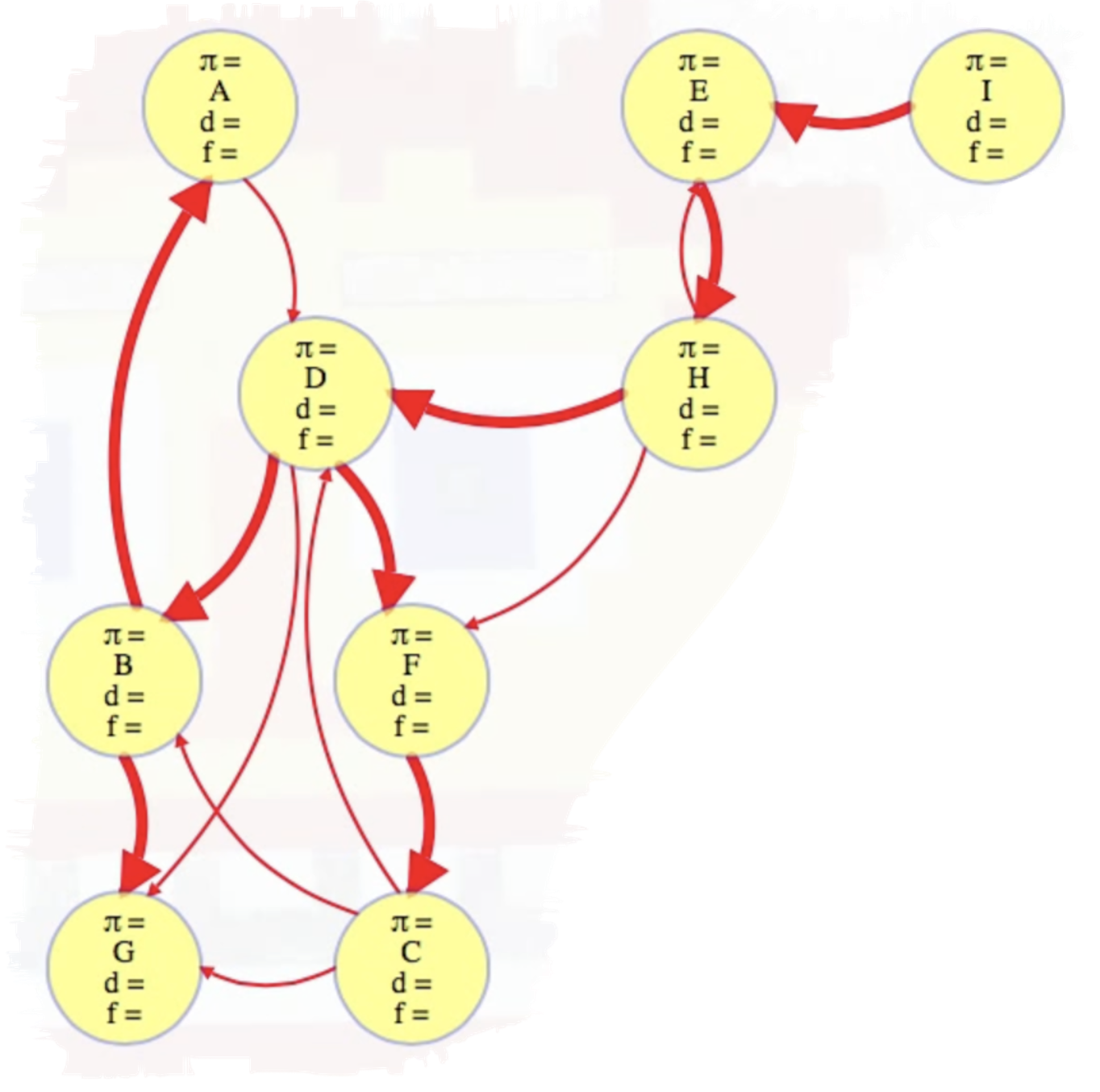
We'll execute top-level searches on vertices in alphabetical order. Doing so yields the following completely searched graph, as illustrated in the linked video at the top of this note:
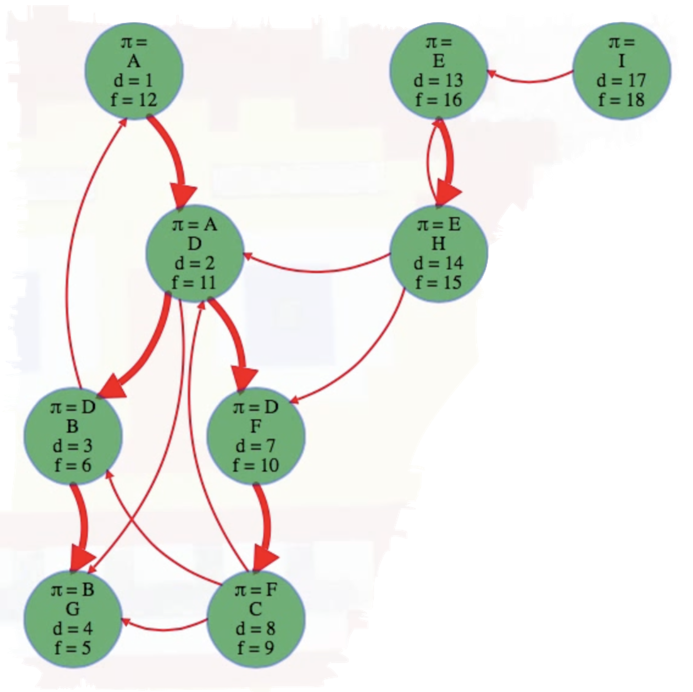
As can be seen above, A, E, and I are the roots of their own depth first search trees in this depth first search forest.
To reproduce the final figure above using code, we can first represent the graph by mapping vertices A through I to 0 through 8, inclusive. It also helps to define a lookup table for ease of reference:
graph = [
[3],
[0, 6],
[1, 3, 6],
[1, 5, 6],
[7],
[2],
[],
[3, 4, 5],
[4],
]
lookup = {
-1: ' ',
0: 'A',
1: 'B',
2: 'C',
3: 'D',
4: 'E',
5: 'F',
6: 'G',
7: 'H',
8: 'I',
}
Now we can write the dfs function to execute a DFS on the entire graph — the inner visit function is where the DFSVertex method is implemented (a reformatting of the output is included at the bottom of the code):
def dfs(graph):
n = len(graph)
discovered = [-1] * n
finished = [-1] * n
pred = [-1] * n
time = 0
def visit(node):
nonlocal time
time += 1
discovered[node] = time
for nbr in graph[node]:
if discovered[nbr] < 0:
pred[nbr] = node
visit(nbr)
time += 1
finished[node] = time
for node in range(n):
if discovered[node] < 0:
visit(node)
return discovered, finished, [ lookup[parent] for parent in pred ]
print(dfs(graph))
"""
( A B C D E F G H I
[ 1, 3, 8, 2, 13, 7, 4, 14, 17], # discovered times
[12, 6, 9, 11, 16, 10, 5, 15, 18], # finished times
[ , D, F, A, , D, B, E, ] # pi values
)
"""
The next two aspects of DFS we will consider, namely parenthesis notation and edge classification are remarked on in greater detail in [24]. The relevant snippets from CLRS are reproduced below (it would likely be helpful to look at these snippets before looking at these topics in the context of the example we've been working through).
Parenthesis theorem (CLRS)
Depth-first search yields valuable information about the structure of a graph. Perhaps the most basic property of depth-first search is that the predecessor subgraph does indeed form a forest of trees, since the structure of the depth-first trees exactly mirrors the structure of recursive calls of DFS-VISIT. That is, if and only if was called during a search of 's adjacency list. Additionally, vertex is a descendant of vertex in the depth-first forest if and only if is discovered during the time in which is gray.
Another important property of depth-first search is that discovery and finish times have parenthesis structure. If the DFS-VISIT procedure were to print a left parenthesis "" when it discovers vertex and to print a right parenthesis "" when it finishes , then the printed expression would be well formed in the sense that the parentheses are properly nested.
The following theorem provides another way to characterize the parenthesis structure.
In any depth-first search of a (directed or undirected) graph , for any two vertices and , exactly one of the following three conditions holds:
- the intervals and are entirely disjoint, and neither nor is a descendant of the other in the depth-first forest,
- the interval is contained entirely within the interval , and is a descendant of in a depth-first tree, or
- the interval is contained entirely within the interval , and is a descendant of in a depth-first tree.
Edge classification (CLRS)
You can obtain important information about a graph by classifying its edges during a depth-first search. For example, Section 20.4 will show that a directed graph is acyclic if and only if a depth-first search yields no "back" edges (Lemma 20.11).
The depth-first forest produced by a depth-first search on graph can contain four types of edges
- Tree edges are edges in the depth-first forest . Edge is a tree edge if was first discovered by exploring edge .
- Back edges are those edges connecting a vertex to an ancestor in a depth-first tree. We consider self-loops, which may occur in directed graphs, to be back edges.
- Forward edges are those nontree edges connecting a vertex to a proper descendant in a depth-first tree.
- Cross edges are all other edges. They can go between vertices in the same depth-first tree, as long as one vertex is not an ancestor of the other, or they can go between vertices in different depth-first trees.
The DFS algorithm has enough information to classify some edges as it encounters them. The key idea is that when an edge is first explored, the color of vertex says something about the edge:
- WHITE indicates a tree edge,
- GRAY indicates a back edge, and
- BLACK indicates a forward or cross edge.
The first case is immediate from the specification of the algorithm. For the second case, observe that the gray vertices always form a linear chain of descendants corresponding to the stack of active DFS-VISIT invocations. The number of gray vertices is 1 more than the depth in the depth-first forest of the vertex most recently discovered. Depth-first search always explores from the deepest gray vertex, so that an edge that reaches another gray vertex has reached an ancestor. The third case handles the remaining possibility.
The entire depth first search from the worked example above can be summarized nicely using parentheses:

An opening parentheses stands for when the depth first search call is made on a vertex, and the closed parentheses stands for when that call exits:
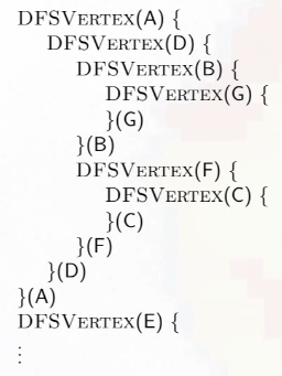
The parentheses are properly nested because the inner recursive calls must complete before the code that called them. A child will always be nested in its parent, and a vertex is only the child of at most one vertex, the one that discovered it.
If we just count the parentheses from the beginning, they will match the discovery and finish times:
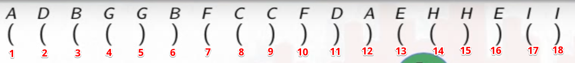
Recall the fully explored graph for reference and comparison:
In CLRS they do two more things. First, they color vertices in the following manner:
- White: Undiscovered
- Gray: Discovered (but unifinished)
- Black: Finished
Second, they classify edges:
- Tree edges (parent to a child): go to an undiscovered vertex
- Back edges (to an ancestor): to a discovered but unfinished vertex (creates a cycle). During DFS, every back edge completes a cycle. Removing back edges from a graph would remove all cycles.
- Forward edges (to a non-child descendant): to a finished vertex discovered after the current vertex. A forward edge is basically an edge that goes to an indirect descendant, not a direct child. For the graph we've been considering, the edge from
DtoGis a forward edge. How can we tell? BecauseGis finished but its discovery time is after that of the current node,D. The vertexGwas discovered and explored during the lifetime ofG— it's a descendant ofDbut not a direct descendant. NodeBis the direct descendant ofD; nodeGis the direct descendant ofB; and nodeGis an indirect descendant ofD. - Cross edges (everything else): to a vertex finished before the current vertex's discovery. It's essentially any edge that's not captured in the edge classifications above. It can go from one branch of a tree to another or even from one tree to another. And there isn't any ancestor or descendant relation between the vertices it links. You can tell because it leads to a vertex that finished before the current vertex was discovered. Its parentheses don't overlap.
If we color our example graph so that tree edges are red, back edges are black, forward edges are blue, and cross edges are green, then we end up with the following:
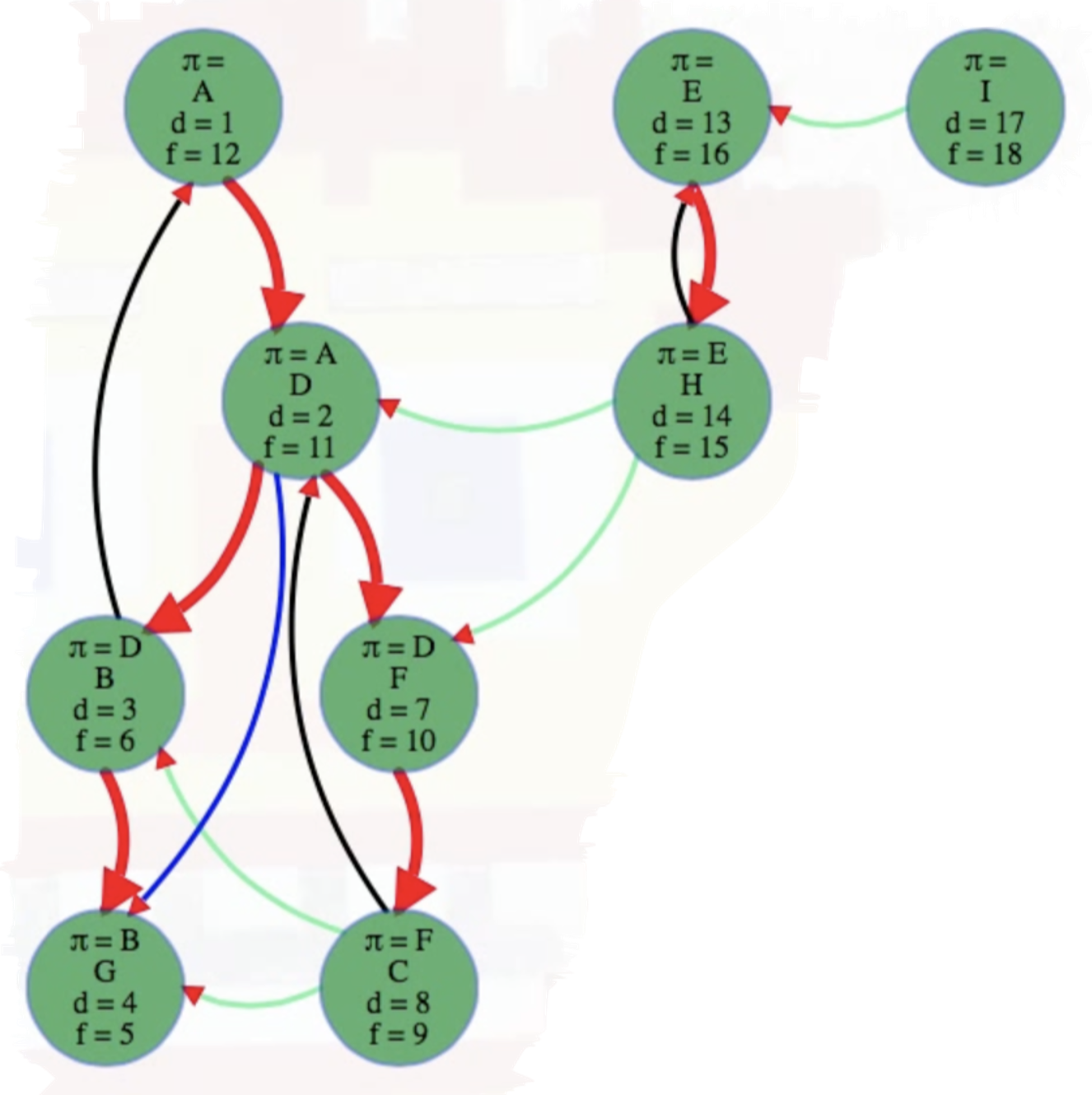
For undirected graphs, we end up seeing each edge twice, once from each vertex. If we classify the edge the first time we see it, then there won't be any forward or cross edges, only tree and back edges.
Unlike breadth first search, if a graph is more connected, then its depth first search trees tend to be taller and more vine-like. If vertices have lots of outgoing edges, then you can keep finding new vertices to explore, and the tree depth can get large. This brings us to a possible implementation hiccup for DFS — for each recursive call, we push variables onto our program's call stack. Different languages have different limits to how deep the call stack can be. A graph with 20,000 vertices might try to make 20,000 nested recursive DFS calls, which can give you a program stack overflow error. To avoid this, we can use our own stack instead of the implicit call stack with recursion.
We can do this in a few ways, but here is one possible manner:
ResetGraph(G)
for v in V
v.pi = nil
v.discovered = -1
v.finished = -1
time = 1
ExploreVertex(u, S)
if (u.discovered < 0)
u.discovered = time++
S.push(u)
for each v such that u -> v
S.push(u -> v)
else if (u.finished < 0)
u.finished = time++
# else: ignore, top level search of finished vertex
ExploreEdge(u -> v, S)
if (v.discovered < 0)
(u -> v).label = "treeEdge"
v.pi = u
ExploreVertex(v, S)
else if (v.finished < 0)
(u -> v).label = "backEdge
else if (v.discovered > u.discovered)
(u -> v).label = "forwardEdge"
else
(u -> v).label = "crossEdge"
DFS(G)
ResetGraph(G)
S = new Stack()
for u in V
S.push(u)
while (not S.isEmpty())
x = S.pop()
if (x.isVertex())
ExploreVertex(x, S)
else
ExploreEdge(x, S)
Let's go through how the pseudocode above is meant to function:
- Line
32: Here, we make a stack where we can push edges and vertices. - Lines
33-36: Push all vertices on to the stack and pop while the stack isn't empty. - Lines
9-13: If we pop an undiscovered vertex, then discover it! Push it again to finish it later, and push its outgoing edges. When we pop it again later, after it's discovered (line14), then finish it (line15). And if we pop an already finished vertex, then just ignore it (line16). That's the equivalent of looping through all vertices but only running depth first search on the undiscovered ones. - Lines
19-28: When we pop an edge from the stack, if it leads to an undiscovered vertex, then it's a tree edge and label it as so (line20) and explore that vertex (line22); otherwise, just label the edge and we're done with it (lines23-28).
In the two lines where we push either all vertices (line 34) or all edges from a vertex (line 13), if we push them in the opposite order that you would normally loop through them in the recursive version of the algorithm, then the version above will give us the same results, same times, edge classifications, etc. It will all be the same as the recursive version. The code above doesn't look quite as clean, but it's a nice parallel to see that while breadth first search explicitly uses a first in first out queue of vertices, depth first search can explicitly use a stack of vertices and edges instead of just implicitly using the program call stack.
If we implement all of the pseudocode above for the iterative version, then we will end up with something like the following (the blocks of code have been highlighted where ordering has intentionally been reversed to ensure the same results as the recursive version):
def dfs_iter(graph):
n = len(graph)
edge_classifications = dict()
discovered = [-1] * n
finished = [-1] * n
pred = [-1] * n
time = 0
def explore_vertex(node):
nonlocal time
if discovered[node] < 0:
time += 1
discovered[node] = time
stack.append(node)
for i in range(len(graph[node]) - 1, -1, -1):
nbr = graph[node][i]
stack.append((node, nbr))
elif finished[node] < 0:
time += 1
finished[node] = time
def explore_edge(edge):
node, nbr = edge
if discovered[nbr] < 0:
edge_classifications[edge] = 'treeEdge'
pred[nbr] = node
explore_vertex(nbr)
elif finished[nbr] < 0:
edge_classifications[edge] = 'backEdge'
elif discovered[nbr] > discovered[node]:
edge_classifications[edge] = 'forwardEdge'
else:
edge_classifications[edge] = 'crossEdge'
stack = []
for node in range(n - 1, -1, -1):
stack.append(node)
while stack:
x = stack.pop()
if not isinstance(x, tuple):
explore_vertex(x)
else:
explore_edge(x)
return discovered, finished, pred, { (lookup[edge[0]], lookup[edge[1]]): edge_classifications[edge] for edge in edge_classifications }
The outcome, formatted manually for the sake of clarity, matches exactly what was produced previously using the recursive approach (the edge classification also matches what we would expect):
"""
( A B C D E F G H I
[ 1, 3, 8, 2, 13, 7, 4, 14, 17], # discovered
[12, 6, 9, 11, 16, 10, 5, 15, 18], # finished
[-1, 3, 5, 0, -1, 3, 1, 4, -1], # predecessors
{ # edge classifications
('A', 'D'): 'treeEdge',
('D', 'B'): 'treeEdge',
('B', 'A'): 'backEdge',
('B', 'G'): 'treeEdge',
('D', 'F'): 'treeEdge',
('F', 'C'): 'treeEdge',
('C', 'B'): 'crossEdge',
('C', 'D'): 'backEdge',
('C', 'G'): 'crossEdge',
('D', 'G'): 'forwardEdge',
('E', 'H'): 'treeEdge',
('H', 'D'): 'crossEdge',
('H', 'E'): 'backEdge',
('H', 'F'): 'crossEdge',
('I', 'E'): 'crossEdge'
}
)
"""
Why is the order reversal in the iterative version important in order to ensure the same results as in the recursive version? Because stacks are LIFO data structures — if we push elements onto the stack in the same order as we would process them recursively, then they will be popped off in reverse order. Consider the worked example we've been dealing with throughout this entire note. If we pushed the vertices A through I onto the stack in that order, then the first vertex popped off would be F, not A. But that's not the desired result! Hence, we push vertices I, H, ... , B, A onto the stack in that order so they are popped in the order A, B, ... , H, I, much as the order they are processed in the recursive version. Similarly, the order in which neighboring vertices are processed needs to be reversed as well; that is, we need to push neighbors onto the stack in reverse order — this ensures that when they are popped off the stack, they are processed in the original order.
Consider a generalized example to fully clarify things:
- Adjacency list: Let's say
uhas neighbors[v1, v2, v3]. - Recursive DFS: Processes
v1, thenv2, thenv3. - Iterative DFS (without reversal):
- Push
v1,v2,v3onto the stack. - Pop and process
v3,v2,v1(reverse order).
- Push
- Iterative DFS (with reversal):
-
Push
v3,v2,v1onto the stack. -
Pop and process
v1,v2,v3(original order).
-
def fn(graph):
def dfs(node):
ans = 0
# do some logic
for neighbor in graph[node]:
if neighbor not in seen:
seen.add(neighbor)
ans += dfs(neighbor)
return ans
seen = {START_NODE}
return dfs(START_NODE)
Examples
LC 547. Number of Provinces (✓)
There are n cities. Some of them are connected, while some are not. If city a is connected directly with city b, and city b is connected directly with city c, then city a is connected indirectly with city c.
A province is a group of directly or indirectly connected cities and no other cities outside of the group.
You are given an n x n matrix isConnected where isConnected[i][j] = 1 if the ith city and the jth city are directly connected, and isConnected[i][j] = 0 otherwise.
Return the total number of provinces.
class Solution:
def findCircleNum(self, isConnected: List[List[int]]) -> int:
def build_adj_list(adj_mat):
graph = defaultdict(list)
n = len(adj_mat)
for node in range(n):
for neighbor in range(node + 1, n):
if isConnected[node][neighbor] == 1:
graph[node].append(neighbor)
graph[neighbor].append(node)
return graph
def dfs(node):
for neighbor in graph[node]:
if neighbor not in seen:
seen.add(neighbor)
dfs(neighbor)
graph = build_adj_list(isConnected)
seen = set()
provinces = 0
for city in range(len(isConnected)):
if city not in seen:
provinces += 1
seen.add(city)
dfs(city)
return provinces
Cities are nodes, connected cities are provinces (i.e., connected components). The idea here is to explore all provinces by starting with each city and seeing how many cities we can explore from that city — every time we have to start a search again from a new city, we increment the number of overall provinces encountered thus far.
LC 200. Number of Islands (✓)
Given an m x n 2D binary grid grid which represents a map of '1's (land) and '0's (water), return the number of islands.
An island is surrounded by water and is formed by connecting adjacent lands horizontally or vertically. You may assume all four edges of the grid are all surrounded by water.
class Solution:
def numIslands(self, grid: List[List[str]]) -> int:
def valid(row, col):
return 0 <= row < m and 0 <= col < n and grid[row][col] == '1'
def dfs(row, col):
for dr, dc in dirs:
next_row, next_col = row + dr, col + dc
neighbor = (next_row, next_col)
if neighbor not in seen and valid(*neighbor):
seen.add(neighbor)
dfs(*neighbor)
m = len(grid)
n = len(grid[0])
dirs = [(-1,0),(1,0),(0,-1),(0,1)]
seen = set()
islands = 0
for i in range(m):
for j in range(n):
node = (i, j)
if node not in seen and grid[i][j] == '1':
islands += 1
seen.add(node)
dfs(*node)
return islands
Each "island" is a connected component — our job is to count the total number of connected components. The traversal is a fairly standard DFS traversal on a grid-like graph.
LC 1466. Reorder Routes to Make All Paths Lead to the City Zero (✓)
There are n cities numbered from 0 to n-1 and n-1 roads such that there is only one way to travel between two different cities (this network form a tree). Last year, The ministry of transport decided to orient the roads in one direction because they are too narrow.
Roads are represented by connections where connections[i] = [a, b] represents a road from city a to b.
This year, there will be a big event in the capital (city 0), and many people want to travel to this city.
Your task consists of reorienting some roads such that each city can visit the city 0. Return the minimum number of edges changed.
It's guaranteed that each city can reach the city 0 after reorder.
class Solution:
def minReorder(self, n: int, connections: List[List[int]]) -> int:
roads = set()
def build_adj_list(edge_arr):
graph = defaultdict(list)
for node, neighbor in edge_arr:
roads.add((node, neighbor))
graph[node].append(neighbor)
graph[neighbor].append(node)
return graph
def dfs(node):
ans = 0
for neighbor in graph[node]:
if neighbor not in seen:
seen.add(neighbor)
if (node, neighbor) in roads:
ans += 1
ans += dfs(neighbor)
return ans
graph = build_adj_list(connections)
seen = {0}
return dfs(0)
This is a tough one to come up with if you haven't seen it before. The solution approach above is quite clever. The idea is to build an undirected graph in the form of an adjacency list and then to conduct a DFS from node 0, which means every edge we encounter is necessarily leading away from 0; hence, if that edge appeared in the original road configuration, roads, then we know that road's direction must be changed so that it faces toward node 0 instead of away.
LC 841. Keys and Rooms (✓)
There are N rooms and you start in room 0. Each room has a distinct number in 0, 1, 2, ..., N-1, and each room may have some keys to access the next room.
Formally, each room i has a list of keys rooms[i], and each key rooms[i][j] is an integer in [0, 1, ..., N-1] where N = rooms.length. A key rooms[i][j] = v opens the room with number v.
Initially, all the rooms start locked (except for room 0).
You can walk back and forth between rooms freely.
Return true if and only if you can enter every room.
class Solution:
def canVisitAllRooms(self, rooms: List[List[int]]) -> bool:
def dfs(node):
for neighbor in rooms[node]:
if neighbor not in seen:
seen.add(neighbor)
dfs(neighbor)
seen = {0}
dfs(0)
return len(seen) == len(rooms)
It's quite nice that the given input, rooms, is already in the form of an adjacency list (as an index array). The key insight is to realize that we can use our seen set to determine whether or not all rooms have been visited after conducting a DFS from node 0 (i.e., room 0); that is, if seen is the same length as rooms after the DFS from node 0, then we can say it's possible to visit all rooms (otherwise it's not).
LC 1971. Find if Path Exists in Graph (✓)
There is a bi-directional graph with n vertices, where each vertex is labeled from 0 to n - 1 (inclusive). The edges in the graph are represented as a 2D integer array edges, where each edges[i] = [ui, vi] denotes a bi-directional edge between vertex ui and vertex vi. Every vertex pair is connected by at most one edge, and no vertex has an edge to itself.
You want to determine if there is a valid path that exists from vertex start to vertex end.
Given edges and the integers n, start, and end, return true if there is a valid path from start to end, or false otherwise.
class Solution:
def validPath(self, n: int, edges: List[List[int]], source: int, destination: int) -> bool:
def build_adj_list(edge_arr):
graph = defaultdict(list)
for node, neighbor in edge_arr:
graph[node].append(neighbor)
graph[neighbor].append(node)
return graph
def dfs(node):
if node == destination:
return True
for neighbor in graph[node]:
if neighbor not in seen:
seen.add(neighbor)
if dfs(neighbor):
return True
return False
graph = build_adj_list(edges)
seen = {source}
return dfs(source)
The solution above is a direct application of a DFS traversal. The hardest part is arguably coming up with an effective way of writing the dfs function. It's better not to rely on a nonlocal variable unless we really need to. The idea is that we should stop searching if we encounter a node whose value is equal to the destination. If that is not the case, then we try to explore further. If our DFS comes up empty, then we return False, and that will propagate back up the recursion chain.
LC 323. Number of Connected Components in an Undirected Graph (✓)
You have a graph of n nodes. You are given an integer n and an array edges where edges[i] = [ai, bi] indicates that there is an edge between ai and bi in the graph.
Return the number of connected components in the graph.
class Solution:
def countComponents(self, n: int, edges: List[List[int]]) -> int:
def build_adj_list(edge_arr):
graph = defaultdict(list)
for node, neighbor in edge_arr:
graph[node].append(neighbor)
graph[neighbor].append(node)
return graph
def dfs(node):
for neighbor in graph[node]:
if neighbor not in seen:
seen.add(neighbor)
dfs(neighbor)
graph = build_adj_list(edges)
seen = set()
cc = 0
for node in range(n):
if node not in seen:
cc += 1
seen.add(node)
dfs(node)
return cc
Counting the number of connected components in a graph via DFS traversal is a very common task. Sometimes the nature of the connected components may be obfuscated at first (i.e., we have to come up with a way to first model the connections and then determine the number of connected components), but that is not the case here.
One thing worth noting in the solution above is how we deftly take care of the case where a node is not represented in the original edge list we're provided. We simply increment the count of the number of connected components, cc, as soon as we encounter a node we have not seen before, and we do this for all n nodes. For nodes that are not connected to any other nodes, are dfs function effectively does not execute.
LC 695. Max Area of Island (✓)
Given a non-empty 2D array grid of 0's and 1's, an island is a group of 1's (representing land) connected 4-directionally (horizontal or vertical.) You may assume all four edges of the grid are surrounded by water.
Find the maximum area of an island in the given 2D array. (If there is no island, the maximum area is 0.)
class Solution:
def maxAreaOfIsland(self, grid: List[List[int]]) -> int:
def valid(row, col):
return 0 <= row < m and 0 <= col < n and grid[row][col] == 1
def dfs(row, col):
connected_area = 0
for dr, dc in dirs:
next_row, next_col = row + dr, col + dc
next_node = (next_row, next_col)
if valid(*next_node) and next_node not in seen:
seen.add(next_node)
connected_area += 1 + dfs(*next_node)
return connected_area
m = len(grid)
n = len(grid[0])
dirs = [(-1,0),(1,0),(0,1),(0,-1)]
seen = set()
max_area = 0
for i in range(m):
for j in range(n):
if (i, j) not in seen and grid[i][j] == 1:
seen.add((i, j))
max_area = max(max_area, 1 + dfs(i, j))
return max_area
The idea here is to basically find the largest connected component.
LC 2368. Reachable Nodes With Restrictions (✓)
There is an undirected tree with n nodes labeled from 0 to n - 1 and n - 1 edges.
You are given a 2D integer array edges of length n - 1 where edges[i] = [ai, bi] indicates that there is an edge between nodes ai and bi in the tree. You are also given an integer array restricted which represents restricted nodes.
Return the maximum number of nodes you can reach from node 0 without visiting a restricted node.
Note that node 0 will not be a restricted node.
class Solution:
def reachableNodes(self, n: int, edges: List[List[int]], restricted: List[int]) -> int:
restricted = set(restricted)
def build_adj_list(edge_arr):
graph = defaultdict(list)
for node, neighbor in edge_arr:
if node not in restricted and neighbor not in restricted:
graph[node].append(neighbor)
graph[neighbor].append(node)
return graph
def dfs(node):
for neighbor in graph[node]:
if neighbor not in seen and neighbor not in restricted:
seen.add(neighbor)
dfs(neighbor)
graph = build_adj_list(edges)
seen = {0}
dfs(0)
return len(seen)
The idea behind the solution above is to start by ensuring our graph only has valid nodes. This means getting rid of all edges that contain one (or both) nodes from the restricted list, which we start by "setifying" in order to make it possible to have lookups.
It's worth reflecting on why it behooves us to get rid of an edge when one of its nodes is from the restricted set. If the node in the restricted is the source, then there's no way to get to its destination. If the restricted node is the destination, then we will not go there from the source. Whatever the case, it is a waste of time and space to consider edges that have one (or both) nodes from the restricted set.
At the end, the number of nodes reached from 0 is the length of the set seen, which is why we return len(seen). We could just as well kept track of the number of visited nodes by just using the dfs function itself:
class Solution:
def reachableNodes(self, n: int, edges: List[List[int]], restricted: List[int]) -> int:
restricted = set(restricted)
def build_adj_list(edge_arr):
graph = defaultdict(list)
for node, neighbor in edge_arr:
if node not in restricted and neighbor not in restricted:
graph[node].append(neighbor)
graph[neighbor].append(node)
return graph
def dfs(node):
ans = 0
for neighbor in graph[node]:
if neighbor not in seen and neighbor not in restricted:
seen.add(neighbor)
ans += 1 + dfs(neighbor)
return ans
graph = build_adj_list(edges)
seen = {0}
return dfs(0) + 1
LC 1020. Number of Enclaves (✓) ★★★
You are given an m x n binary matrix grid, where 0 represents a sea cell and 1 represents a land cell.
A move consists of walking from one land cell to another adjacent (4-directionally) land cell or walking off the boundary of the grid.
Return the number of land cells in grid for which we cannot walk off the boundary of the grid in any number of moves.
class Solution:
def numEnclaves(self, grid: List[List[int]]) -> int:
def valid(row, col):
return 0 <= row < m and 0 <= col < n and grid[row][col] == 1
def process_perimeter(mat):
first_row = 0
last_row = m - 1
first_col = 0
last_col = n - 1
boundary_lands = set()
for row in [ first_row, last_row ]:
for col in range(n):
if mat[row][col] == 1:
boundary_lands.add((row, col))
for col in [ first_col, last_col ]:
for row in range(1, m - 1):
if mat[row][col] == 1:
boundary_lands.add((row, col))
return boundary_lands
def dfs(row, col):
ans = 0
for dr, dc in dirs:
next_row, next_col = row + dr, col + dc
if valid(next_row, next_col) and (next_row, next_col) not in seen:
seen.add((next_row, next_col))
ans += 1 + dfs(next_row, next_col)
return ans
m = len(grid)
n = len(grid[0])
dirs = [(1,0),(-1,0),(0,1),(0,-1)]
seen = set()
enclaves = 0
boundary_lands = process_perimeter(grid)
for boundary_land in boundary_lands:
seen.add(boundary_land)
dfs(*boundary_land)
for i in range(m):
for j in range(n):
if (i, j) not in seen and grid[i][j] == 1:
seen.add((i, j))
enclaves += 1 + dfs(i, j)
return enclaves
The solution above could almost certainly be improved, but it captures the core idea for almost any effective solution to this problem — we need to pre-process to identify all land cells that reside on the boundary. A DFS from each of those cells should be used to identify invalid land cells. There are a few ways of doing this — we could mutate the input grid by letting our DFS mark all boundary land cells and invalid connected land cells with 0 or some other value. Then we simply need to count the number of cells with 1 in them. The following solution is much more optimized for this kind of approach:
class Solution:
def numEnclaves(self, grid: List[List[int]]) -> int:
def valid(row, col):
return 0 <= row < m and 0 <= col < n and grid[row][col] == 1
def process_perimeter(mat):
first_row = 0
last_row = m - 1
first_col = 0
last_col = n - 1
for row in [ first_row, last_row ]:
for col in range(n):
if mat[row][col] == 1:
dfs(row, col)
for col in [ first_col, last_col ]:
for row in range(1, m - 1):
if mat[row][col] == 1:
dfs(row, col)
def dfs(row, col):
grid[row][col] = 0
for dr, dc in dirs:
next_row, next_col = row + dr, col + dc
if valid(next_row, next_col):
dfs(next_row, next_col)
m = len(grid)
n = len(grid[0])
dirs = [(1,0),(-1,0),(0,1),(0,-1)]
process_perimeter(grid)
enclaves = 0
for i in range(m):
for j in range(n):
enclaves += grid[i][j]
return enclaves
LC 2192. All Ancestors of a Node in a Directed Acyclic Graph (✓)
You are given a positive integer n representing the number of nodes of a Directed Acyclic Graph (DAG). The nodes are numbered from 0 to n - 1 (inclusive).
You are also given a 2D integer array edges, where edges[i] = [fromi, toi] denotes that there is a unidirectional edge from fromi to toi in the graph.
Return a list answer, where answer[i] is the list of ancestors of the ith node, sorted in ascending order.
A node u is an ancestor of another node v if u can reach v via a set of edges.
class Solution:
def getAncestors(self, n: int, edges: List[List[int]]) -> List[List[int]]:
def build_rev_adj_list(edge_arr):
graph = defaultdict(list)
for node, neighbor in edge_arr:
graph[neighbor].append(node)
return graph
def dfs(node, visited):
for neighbor in graph[node]:
if neighbor not in visited:
visited.add(neighbor)
dfs(neighbor, visited)
return visited
graph = build_rev_adj_list(edges)
return [ sorted(list(dfs(node, set()))) for node in range(n) ]
This is a fun one. The key idea is to invert or reverse the edge directions and then perform a DFS from each node, 0 through n - 1, inclusive, to determine what the ancestors are for each node. Why does this work? Because the ancestors of a target node are whatever nodes have edges that lead to the target node; hence, executing a DFS from the target node once edges have been inverted gives us all ancestral nodes for the target node.
LC 990. Satisfiability of Equality Equations (✓) ★★★
Given an array equations of strings that represent relationships between variables, each string equations[i] has length 4 and takes one of two different forms: "a==b" or "a!=b". Here, a and b are lowercase letters (not necessarily different) that represent one-letter variable names.
Return true if and only if it is possible to assign integers to variable names so as to satisfy all the given equations.
class Solution:
def equationsPossible(self, equations: List[str]) -> bool:
def build_graph(edges):
graph = defaultdict(list)
for equation in edges:
if equation[1] == '=':
node = equation[0]
neighbor = equation[3]
graph[node].append(neighbor)
graph[neighbor].append(node)
return graph
def dfs(node, label):
if label_lookup[node] == -1:
label_lookup[node] = label
for neighbor in graph[node]:
dfs(neighbor, label)
graph = build_graph(equations)
label_lookup = { chr(i): -1 for i in range(97, 122 + 1) }
for char in 'abcdefghijklmnopqrstuvwxyz':
dfs(char, ord(char))
for equation in equations:
if equation[1] == '!':
if label_lookup[equation[0]] == label_lookup[equation[3]]:
return False
return True
Equation problems that require being interpreted as graphs are never very intuitive and always require some creativity. The solution editorial for this problem is quite good and highlights one slick way of approach this problem with DFS as the underlying mechanism for driving the solution logic.
The key idea is to treat each possible variable (a through z) as a node and then to use the provided equations where == is the comparison to essentially label all equal variables in the same way (i.e., it's like we're assigning a number or color to each node in a connected component). Once this has been done, we process all equations where != is the comparison operator — if the nodes that cannot be equal are in separate components (i.e., they have different labels), then we are fine; if, however, two nodes cannot be equal but they share the same label, then this means they must also be equal to other (a contradiction).
LC 1905. Count Sub Islands★★★
You are given two m x n binary matrices grid1 and grid2 containing only 0's (representing water) and 1's (representing land). An island is a group of 1's connected 4-directionally (horizontal or vertical). Any cells outside of the grid are considered water cells.
An island in grid2 is considered a sub-island if there is an island in grid1 that contains all the cells that make up this island in grid2.
Return the number of islands in grid2 that are considered sub-islands.
class Solution:
def countSubIslands(self, grid1: List[List[int]], grid2: List[List[int]]) -> int:
def valid(row, col):
return 0 <= row < m and 0 <= col < n and grid2[row][col] == 1
def dfs(row, col):
if not valid(row, col):
return True
grid2[row][col] = 0
is_subisland = grid1[row][col] == 1
for dr, dc in dirs:
is_subisland &= dfs(row + dr, col + dc)
return is_subisland
m = len(grid2)
n = len(grid2[0])
dirs = [(-1, 0), (1, 0), (0, -1), (0, 1)]
sub_islands = 0
for i in range(m):
for j in range(n):
if grid2[i][j] == 1:
if dfs(i, j):
sub_islands += 1
return sub_islands
The approach above is easier to explain if we generously add comments to the code:
class Solution:
def countSubIslands(self, grid1: List[List[int]], grid2: List[List[int]]) -> int:
def valid(row, col):
return 0 <= row < m and 0 <= col < n and grid2[row][col] == 1
def dfs(row, col):
# early return True if DFS hits out-of-bounds cell or non-island/water cell (0) in grid2
# Boundary cells: When the DFS reaches the boundary of the island (i.e., a cell outside the
# grid or a non-island/water cell), it should not cause the island to be disqualified as a sub-island
# Island check: The goal is to verify that all 1s in the connected component we're exploring in grid2
# correspond to 1s in grid1; the DFS should stop (return True) if it hits water or goes out of bounds
# because these conditions do not invalidate the sub-island
# Summary: Essentially, the "if not valid(row, col): return True" condition ensures the DFS only
# continues exploring valid island cells within grid2's bounds and stops when it reaches the edge
# of the island or goes out of bounds. Returning True here is the equivalent of saying, "This path
# is fine, keep checking the rest of the island."
if not valid(row, col):
return True
grid2[row][col] = 0 # mark cell as visited
is_subisland = grid1[row][col] == 1 # does the land cell in grid2 correspond to a land cell in grid1?
for dr, dc in dirs:
is_subisland &= dfs(row + dr, col + dc)
return is_subisland
m = len(grid2)
n = len(grid2[0])
dirs = [(-1, 0), (1, 0), (0, -1), (0, 1)]
sub_islands = 0
for i in range(m):
for j in range(n):
if grid2[i][j] == 1: # start exploring an island in grid2
if dfs(i, j): # all land cells in grid2 correspond to land cells in grid1
sub_islands += 1 # (out of bounds and non-island/water cells do not invalidate sub-islands)
return sub_islands
Time: . Let and represent the number of rows and columns, respectively. We iterate over all rows and columns in grid2.
Space: . The main space cost is from the recursive call stack.
LC 947. Most Stones Removed with Same Row or Column★★
On a 2D plane, we place n stones at some integer coordinate points. Each coordinate point may have at most one stone.
A stone can be removed if it shares either the same row or the same column as another stone that has not been removed.
Given an array stones of length n where stones[i] = [xi, yi] represents the location of the ith stone, return the largest possible number of stones that can be removed.
class Solution:
def removeStones(self, stones: List[List[int]]) -> int:
def build_graph(coords):
graph = defaultdict(list)
for i in range(len(coords)):
x1, y1 = coords[i]
for j in range(i + 1, len(coords)):
x2, y2 = coords[j]
if x1 == x2 or y1 == y2:
graph[(x1, y1)].append((x2, y2))
graph[(x2, y2)].append((x1, y1))
return graph
def dfs(row, col):
for neighbor in graph[(row, col)]:
if neighbor not in seen:
seen.add(neighbor)
dfs(*neighbor)
graph = build_graph(stones)
seen = set()
connected_components = 0
for stone in stones:
stone = tuple(stone)
if stone not in seen:
connected_components += 1
seen.add(stone)
dfs(*stone)
return len(stones) - connected_components
The solution editorial for this problem is quite good in terms of highlighting the core concepts needed for implementing the DFS approach:
-
Connected components: Two stones are considered "connected" if they share a row or column, but this connection extends beyond just pairs of stones. If stone A is connected to stone B and stone B is connected to stone C, then all three stones form part of the same group, even if A and C don’t directly share a row or column. This concept is akin to connected components in graph theory, where a connected component is a group of nodes where you can reach any node from any other node in the group.
-
Calculating remaining stones: Since every stone in a connected component shares a row or column with at least one other stone, we can remove all but one stone. The remaining stone cannot be removed as it no longer shares coordinates with any other stone, having eliminated all others in its component. Therefore, if our 2-D plane contains multiple connected components, each can be reduced to a single stone. The maximum number of stones that can be removed can be mathematically expressed as:
Max removable stones = Total stones - Number of connected components
The implementation thus boils down to two parts:
- Represent the stones as a graph.
- Count the number of connected components in this graph.
For the first part, we can utilize an adjacency list, where for each stone, we maintain a list of all other stones it's connected to (i.e., shares a row or column with). Unfortunately, there does not seem to be a more efficient way of doing this than by means of an approach. We can use DFS for the second part, as shown above.
Time: . Let be the number of stones. We iterate over all pairs of stones.
Space: . All stones could be on the same row or column.
DFS (iterative)
Remarks
Assume the nodes are numbered from 0 to n - 1 and the graph is given as an adjacency list. Depending on the problem, you may need to convert the input into an equivalent adjacency list before using the templates.
def fn(graph):
stack = [START_NODE]
seen = {START_NODE}
ans = 0
while stack:
node = stack.pop()
# do some logic
for neighbor in graph[node]:
if neighbor not in seen:
seen.add(neighbor)
stack.append(neighbor)
return ans
Examples
TBD
Topological sort (Kahn's algorithm)
Number of paths between nodes in a DAG
A single-source shortest path (SSSP) algorithm tries to find the shortest path from a start node to all other nodes in the graph. We can make a similar assessment concerning the number of paths between nodes in a DAG: we want to find the number of paths from some start node to all other nodes in the DAG.
A template for doing so is as follows:
# T: O(V + E); S: O(V)
def num_paths(graph, start):
n = len(graph)
top_order = topological_sort(graph)
count = [0] * n
count[start] = 1
for node in top_order:
for neighbor in graph[node]:
count[neighbor] += count[node]
return count
This template works as follows:
- Perform topological sort: Use the topological sort template (i.e., Kahn's algorithm) to find a topological ordering of the nodes (this assumes our graph is a DAG).
- Initialize path count array: Create an array or map
countwherecount[v]will store the number of path fromstarttotarget, wheretargetis an arbitrary node in the DAG. Initializecount[start] = 1since there is exactly one path fromstartto itself. Then initializecount[target] = 0for all other nodestarget != start. - Process nodes in topological order: Iterate through each node
nodein the topologically sorted order. For each outgoing edge[node, neighbor], update the path count forneighborby adding the current path count ofnode:count[neighbor] += count[node]. Importantly, this ensures that by the time we processneighbor, all possible paths leading tonodehave already been accounted for. - Retrieve result: After processing all nodes,
countwill contain the total number of distinct paths fromstartto every other node in the DAG. If we are only interested in the number of distinct paths fromstartto a specific other node,target, then we can returncount[target]instead ofcount.
As an example, consider the DAG
S → A → T
S → B → T
A → B
which can be represented as an adjacency list as follows (where S, A, B, and T are mapped to 0, 1, 2, and 3, respectively):
graph = {
0: [1, 2], # (S, A), (S, B)
1: [2, 3], # (A, B), (A, T)
2: [3], # (B, T)
3: []
}
Running the template code on this graph with S as the start node yields the following: [1, 1, 2, 3], which means there's 1 path from S to itself, 1 path from S to A, 2 paths from S to B, and 3 paths from S to T.
SSSPs on DAGs (shortest and longest paths)
Given a start node, we can find single-source shortest paths in (weighted) DAGs by first generating a topological ordering of the nodes (e.g., using Khan's algorithm, as provided in the template) and then relaxing the edges of all nodes in the graph, following the ordering, where both of these steps can be done in linear time proportional to the size of the graph:
# T: O(V + E); S: O(V + E)
def shortest_path_DAG(graph, start):
n = len(graph)
top_order = topological_sort(graph)
distances = [float('inf')] * n
distances[start] = 0
for node in top_order:
for neighbor, weight in graph[node]:
if distances[node] + weight < distances[neighbor]: # relax edge 'node -> neighbor' with 'weight'
distances[neighbor] = distances[node] + weight
return distances
The returned distances array will contain the length of the shortest path from start to each node. In the case of DAGs, since there are no cycles, we can also find single-source longest paths by simply negating the weight of each edge, finding the shortest path, and then negating the results:
# T: O(V + E); S: O(V + E)
def longest_path_DAG(graph, start):
n = len(graph)
top_order = topological_sort(graph)
distances = [float('inf')] * n
distances[start] = 0
for node in top_order:
for neighbor, weight in graph[node]:
weight = -weight
if distances[node] + weight < distances[neighbor]: # relax edge 'node -> neighbor' with 'weight'
distances[neighbor] = distances[node] + weight
distances = [ -distance for distance in distances]
return distances
In both cases, note that our original template code for producing a topological ordering needs to be slightly modified where we traverse neighboring nodes: the line for neighbor in graph[node]: needs to be changed to for neighbor, _ in graph[node]: since tuples are now stored in the graph instead of individual nodes (each node's edge weight must be recorded). Additionally, before trying to report a shortest or longest path in a DAG, we need to ensure a topological ordering was actually produced (i.e., no cycle was found for whatever graph we're considering).
William Fiset's video on shortest/longest paths in DAGs provides a nice example of a weighted DAG:
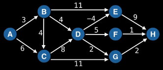
We can map the labelled nodes A, ... , H to 0, ..., 8, respectively, whereby we can then represent the graph as follows:
graph = {
0: [(1, 3), (2, 6)],
1: [(2, 4), (3, 4), (4, 11)],
2: [(3, 8), (6, 11)],
3: [(4, -4), (5, 5), (6, 2)],
4: [(7, 9)],
5: [(7, 1)],
6: [(7, 2)],
7: []
}
Running the code snippets above for shortest and longest paths, where A is the start node, gives us the following:
# A B C D E F G H
[0, 3, 6, 7, 3, 12, 9, 11] # shortest path from node A to each node
[0, 3, 7, 15, 14, 20, 18, 23] # longest path from node A to each node
Inventing a topological sort algorithm (Kahn's algorithm)
The following observations and algorithms in pseudocode appear in Kahn's Algorithm for Topological Sorting video on the "Algorithms with Attitude" YouTube channel.
The linked video above does a fantastic job illustrating how one might "invent" a way to find a topological ordering for a graph by a series of observations and iterative improvements. The final observation and algorithm reflect the template for finding topological orderings.
Observation and algorithm (1):
- A vertex with no incoming edges can go first (this suggests the in-degree for graph nodes will play a part in developing an effective algorithm) — recall that a directed edge
A -> BmeansB"depends" onAin the sense thatAmust come beforeBin whatever eventual topological ordering of the nodes we produce. - A DAG must contain a vertex with no incoming edges or else we are dead in the water from the beginning (if no such node existed, then this would mean every node has a dependency and thus we do not have a sensible starting point); fortunately, by definition, a DAG has to have at least one node with no incoming edges (otherwise we would have a cycle).
- If you want to find a vertex with an in-degree of
0(i.e., no incoming edges), then start at an arbitrary vertex and follow a path of incoming edges backwards:- If we get to a vertex with no incoming edges, then great!
- If not, then once we've gone back edges in a graph with vertices, then we must be repeating vertices which means we must have a cycle.
The observations above make it possible for us to come up with a first stab at an algorithm:
Topsort(G)
while G isn't empty
find u in V with no incoming edges
put u next in the topological ordering
remove u and all its outgoing edges from G
Observation and algorithm (2):
The algorithm above works and its efficiency depends on implementation details. If we get the graph as an outgoing adjacency list (the usual graph representation for search algorithms we are often given or need to build), then finding a vertex with no incoming edges might take a while. And we do that once for each vertex we put in the ordering. To make it fast, maybe we don't need to do that from scratch after every vertex.
To start the algorithm in time linear for the size of the graph, we can create an incoming list for each vertex. With those incoming adjacency lists, we can find all vertices with no incoming edges, and those are the vertices that can go first. We can grab all of those vertices to make an ordered list of vertices that are ready to go, A and C in the sample graph in the video.
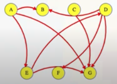
If we let A go first, then we use its outgoing adjacency list to figure out which edges to delete from the incoming adjacency lists of B, then E. When we delete A's edge to vertex E, we see it is E's last incoming edge so we can add E to our growing ordered list. Finally, we delete A from G's incoming list, and we finally delete A from the graph. We continue through the list this way, where each time we get to a vertex, we look at its outgoing edges, delete them from the corresponding incoming edge lists, and if it's the last incoming edge for a vertex, then we can add that vertex to our ordered list.
To summarize this second set of observations:
- There's no need to start from scratch each time:
- Compute incoming adjacency list just once to start
- Grab a set of all 0 in-degree vertices
- Find new 0 in-degree vertices as vertices are removed from the graph
If we incorporate the new observations into pseudocode for an improved algorithm, then we will have something like the following:
Topsort(G)
create incoming edge adjacency list for each vertex (time linear in the graph size)
S = ordered list
add all vertices with no incoming edges to S (order V time)
while not done with S
consider next vertex u from S
put u next in the topological ordering
while removing u and its outgoing edges from G
if vertex v's incoming edge becomes empty
add v to S
This algorithm still follows the idea of the first one, but it's a bit more efficient in its implementation because it decreases some of the repeated work.
Observation and algorithm (3):
Because of some of the changes we just made to the algorithm, we don't need to delete the vertex u from the graph anymore. We just need to delete it from the incoming adjacency lists it is in. We can imagine using those lists that we created at the start of the algorithm as working space while the outgoing lists don't have to change at all.
Also, that first round of changes introduced a bit of clutter. We don't need to have one ordered list of vertices that are ready to go and another for our topological order, especially since both of them are in the same order. We can drop the extra list.
The observations above are really in service of cleaning things up a bit. To summarize:
- Remove vertices from incoming adjacency lists, not from the graph as a whole
- No need to keep two different ordered sets, with the same order
Topsort(G)
create incoming edge adjacency list for each vertex (time linear in the graph size)
S = ordered list
add all vertices with no incoming edges to S (order V time)
while not done with S
consider next vertex u from S
for each outgoing edge u -> v
remove u from v's incoming list
if v's incoming list is empty
add v to S
Observation and algorithm (4, final algorithm):
Can we do better? How do we really use those incoming lists? The only thing we use each incoming list for is to see if it's empty. We're just keeping these perfect lists, deleting exactly the right edge from each, in order to see if it's empty. We never use the list contents, only its size. So how about we just track the size? Instead of incoming adjacency lists, track in-degrees and decrement them instead of deleting edges. If the in-degree goes to 0, then add them to the list. That's the whole algorithm.
In summary: We don't care what the incoming edges are, only the in-degree.
Topsort(G)
find inDegree for each vertex
S = ordered list
add all vertices with no incoming edges to S
while not done with S
consider next vertex u from S
for each outgoing edge u -> v
decrement v's inDegree
if v's inDegree is 0
add v to S
Comments: Finding all in-degrees takes linear time in the size of the graph. Over the course of the entire algorithm, each vertex is added to the ordered list at most once, either at the start (if it has no incoming edges) or when its in-degree gets decremented to 0. Each vertex in the list is considered at most once, and each edge from the vertex causes at most one constant-time decrement. So the algorithm takes time linear in the graph size.
Something to note when developing this algorithm: What if you had made those last changes to deal with in-degrees instead of incoming lists but kept the separate topological order alongside the ordered list?
Topsort(G)
find inDegree for each vertex
S = ordered list
add all vertices with no incoming edges to S
while not done with S
consider next vertex u from S
#highlight-next-line
put u next in the topological ordering # add this back
for each outgoing edge u -> v
decrement v's inDegree
if v's inDegree is 0
add v to S
The algorithm still runs in linear time. What if you replaced your ordered list with a queue or even a stack? It still works. And still in linear time. This version, where S is a stack, uses the order that things were removed from the stack, but what if we used the order where things went into the stack? It still works and in linear time.
What about cycles?
What if the directed graph we run Kahn's algorithm on has a cycle? Then we won't find a topological ordering, which doesn't exist for a graph with cycles. But what happens if we run Kahn's algorithm anyway? The algorithm won't ever decrement the in-degree of any vertex in a cycle to 0, and vertices reachable from cycles won't ever get to in-degree 0 either.
The list returned by the algorithm will only include vertices that aren't in or reachable from any cycle. We can just check the size of the returned list to see if we have the whole graph or not. If not, then it depends on why we were trying to find a topological ordering in the first place before we can figure out what we should do next.
# T: O(V + E); S: O(V + E)
def topological_sort(graph):
n = len(graph) # n-vertex graph provided as an adjacency list
in_degree = [0] * n # incoming degree for each node that will decrease as nodes
for node in range(n): # are 'peeled off' and placed in the generated topological order
for neighbor in graph[node]:
in_degree[neighbor] += 1
deg_zero = [] # nodes that have no incoming edges and are ready to be
for node in range(n): # 'peeled off' and placed in the topological ordering
if in_degree[node] == 0:
deg_zero.append(node)
top_order = []
while deg_zero:
node = deg_zero.pop() # 'peel off' node and
top_order.append(node) # place in topological order
for neighbor in graph[node]:
in_degree[neighbor] -= 1
if in_degree[neighbor] == 0:
deg_zero.append(neighbor)
if len(top_order) != n: # cycle exists if all nodes can't be 'peeled off'
return []
return top_order
Examples
TBD
Topological sort (DFS)
Motivation for DFS-based algorithm for finding a topological sort
The motivation for the DFS-based algorithm for finding a topological sort, as described below, is largely inspired by this video. My goal here is mostly to provide more explanations and working code.
The idea behind Kahn's algorithm for finding a topological sort was to find a vertex that could go first and work from the beginning; of course, we could also try to find something that could go last and work our way towards the first item. To do that, we could modify Kahn's algorithm to work from the back, but that would really just be Kahn's algorithm again in a different way. It might be slightly slower than before because it would first have to convert the graph into an incoming edge adjacency list representation. That incoming vs. outgoing adjacency list is the only non-symmetrical difference between finding the ordering front to back or back to front.
Another way to find a vertex that can go last is to just run depth first search on the outgoing lists until we get to a vertex with no outgoing edges. That vertex can go last. We'll use the same graph from the example exploration in Kahn's algorithm:
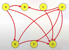
But we can rearrange this graph to make the depth first search tree easier to see (and add space below for an ordering):
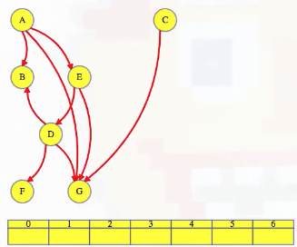
If we run depth first search alphabetically, then we will start with vertex A, and then we find vertex B along a tree edge (edges will be colored according to the color scheme used when first discussing DFS: tree edges (red), back edges (black), forward edges (blue), cross edges (green)). The vertex B has no outgoing edges so it can go last in our topological order:
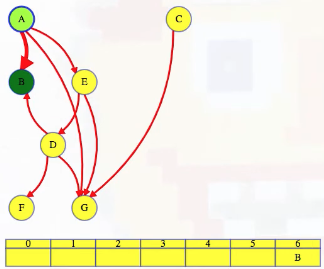
Our depth first search finishes B and returns to A, which has two other outgoing edges. If we want to, we can continue our depth first search looking for other vertices that have no outgoing edges, but let's stop for just a second and think about what the edges from vertex A actually mean. In the graph above, A has edges to B, E, and G, so A has to go before each of those vertices in the topological order. Even more than that, A has to go before any vertex that it can reach in the entire graph, either because it has a direct edge to them or because it has a longer path to them (e.g., vertex D). If A has to precede E, and E has to precede D, then A has to precede D. But what vertices are reachable from A? Exactly those that we will reach when we run depth first search on A. Vertex A can go in the topological order as long as it is before everything that is discovered in the course of a depth first search on it. If we continue the search, then we go to E, then D, and we see a cross edge to B, then we go to F, which has no outgoing edges so F can go last (i.e., out of the remaining vertices):
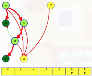
When depth first search returns to D, just like with vertex A, vertex D has to precede everything that it can reach in its depth first search. Continuing that search of D, we get to G, see that it has no outgoing edges, and then we put it after all vertices waiting to be finished:
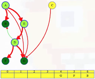
Now when we return to D, all of its outgoing edges have been explored. Everything that has to follow it in the topological ordering, everything it can reach, F and G, have already secured a slot in the ordering after D. So D can go last out of all the unfinished vertices:
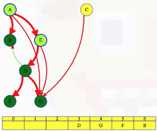
We continue our depth first search. E has a forward edge and then finishes so we can put it in the latest unreserved slot:
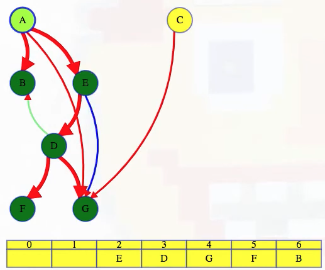
Vertex A has a forward edge to G and then finishes so we can put it in the latest open slot:
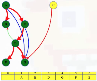
Whenever we finish a vertex, we put in the latest remaining unreserved slot in our topological order. We continue the search on the entire graph, not just the top-level call on vertex A. The top-level search ignores B because it's already searched, but C isn't. But when C finishes, it will add C to the front of the order. Everything else is already explored so all other top-level searches will just move on (i.e., when executing DFS on all nodes of the graph, starting from A gives us everything except C; once C is done, all other vertices will be skipped):
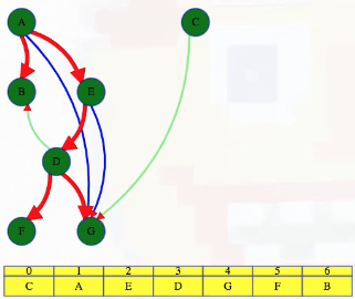
We can now admire our work:
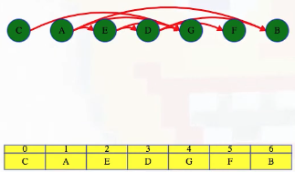
If we repurpose work done in another note (the DFS note on its motivation and a non-recursive way of executing a DFS), then we can define the graph in this example (and a lookup for ease of reference)
graph = [
[1, 4, 6],
[],
[6],
[1, 5, 6],
[3, 6],
[],
[],
]
lookup = {
-1: ' ',
0: 'A',
1: 'B',
2: 'C',
3: 'D',
4: 'E',
5: 'F',
6: 'G',
}
and investigate the non-recursive DFS output:
"""
( A B C D E F G
[ 1, 2, 13, 5, 4, 6, 8], # discovered
[12, 3, 14, 10, 11, 7, 9], # finished
[-1, 0, -1, 4, 0, 3, 3], # predecessors
{ # edge classifications
('A', 'B'): 'treeEdge',
('A', 'E'): 'treeEdge',
('E', 'D'): 'treeEdge',
('D', 'B'): 'crossEdge',
('D', 'F'): 'treeEdge',
('D', 'G'): 'treeEdge',
('E', 'G'): 'forwardEdge',
('A', 'G'): 'forwardEdge',
('C', 'G'): 'crossEdge'
}
)
"""
It's worth noting that the topological sort perfectly aligns with the reverse order in which vertices were finished in the DFS:
# Topological order: C A E D G F B
# finish times
# A B C D E F G <- node correspondence
# [12, 3, 14, 10, 11, 7, 9] <- unordered finish times
# ...
# [14, 12, 11, 10, 9, 7, 3] <- reverse order of finish times
# C A E D G F B <- topological order
We can also confirm all of the edge classifications as they appear in the video:
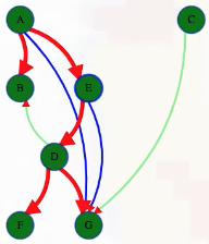
At this point, it's worth asking: What exactly is the algorithm we used here to produce a topological ordering? It's really quite simple:
- Run depth first search on entire graph
- Set the topological order to be the reverse order of vertex finish times
That's it. Because the graph is acyclic, when depth first search on a vertex completes, everything that vertex can reach has been explored — as long as the vertex is before those things in the ordering, it's set. To topologically sort, you don't really need the start or finish times. You could modify depth first search to return the topological ordering directly.
The following graphic does a decent job of giving some intuition as to why this DFS algorithm works for producing a topological ordering when the graph is acyclic:
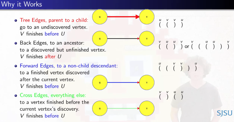
Specifically, using parthensis notation and edge classification (both remarked on in the note for recursive DFS), notice that tree edges, forward edges, and cross edges, the closing parentheses for v come before the closing parentheses for u, which is what we want for all edges u -> v since u -> v implies that v has u as a dependency that needs to be resolved and thus u must come earlier in the ordering. For these three edge types, v will finish before u. So if we take vertices in reverse order of finish time, then any edge from u to v will put v after u, just like we need it to be.
The only problem is back edges, where vertex u would finish before v. But for depth first search on an acyclic graph, there are no back edges since a back edge completes a cycle between a vertex and its ancestor. So don't worry about back edges (unless we're not guaranteed the input graph is acyclic, in which case we need to implement logic for cycle detection).
Two things worth considering in regarde to possible variations of the implementation we've been discussing:
- Subset of vertices: If we only want to consider vertices reachable from a subset of vertices, maybe even a single vertex, then simply modify the top-level depth first search to only search from that subset or that one vertex. The recursive part doesn't change.
- Non-recursive DFS: If we're possibly at risk of a stack overflow, then it may be beneficial to consider an iterative implementation of DFS instead of the recursive implementation.
Finally, it's important to note that if we run our recursive DFS algorithm for finding a topological ordering on a graph that does have cycles, then unlike Kahn's algorithm, our algorithm will return an order including all vertices. Of course, the order returned isn't a topological order (because that doesn't exist for a graph that has cycles), but it can still be helpful due to some special properties that can be exploited based on finishing times. Kosaraju's algorithm for finding strongly connected components (SCCs) makes use of such a non-topological order.
Revised template when input is guaranteed to be a DAG
If it is guaranteed that the input graph is directed and acyclic (i.e., a DAG), then we do not need to track the visiting status of different nodes because a cycle will not be possible by definition:
# T: O(V + E); S: O(V)
def topsort(graph):
n = len(graph)
top_order = []
visited = [False] * n
def dfs(node):
visited[node] = True
for nbr in graph[node]:
if not visited[nbr]:
dfs(nbr)
top_order.append(node)
for node in range(n):
if not visited[node]:
dfs(node)
return top_order
The code above is simply streamlined for contexts where we know for certain that the input graph does not have a cycle.
# T: O(V + E); S: O(V)
def topsort(graph):
n = len(graph) # graph assumed to be provided as an adjacency list of index arrays
top_order = []
visited = [0] * n # 0: unvisited; 1: visiting; 2: visited
def dfs(node):
visited[node] = 1 # mark as visiting
for nbr in graph[node]:
if visited[nbr] == 0: # visit unvisited neighbor
if not dfs(nbr):
return False
elif visited[nbr] == 1: # found a back edge: graph has a cycle
return False
visited[node] = 2 # mark as visited
top_order.append(node) # add node after all descendants have been visited
return True
for node in range(n):
if not visited[node]:
if not dfs(node): # topological sort not possible
return [] # (return empty list)
return top_order
Examples
TBD
Dijkstra (lazy)
How Dijkstra and BFS are similar but strikingly different
William Fiset's YouTube video on Dijkstra is a gem and well worth watching.
Interviewing IO fruitfully compares BFS to Dijkstra and highlights the differences and explains the motivation (paraphrasing to follow): BFS is easier than Dijkstra because we encounter the nodes ordered by distance (with BFS, it's as if we have a weighted graph where all edge weights equal 1). Hence, in BFS, we assign the correct distance to nodes as soon as we reach them for the first time (as a neighbor of the current node), and this happens when we add them to the queue. Thus, in BFS, every node in the queue already has the correct shortest distance. This is not the case in Dijkstra; specifically, especially in the case of lazy Dijkstra, which is the approach most people use, we may find some initial path to a node and later on find a shorter path.
Concrete example of how we can find some initial path to a node and later on find a shorter path
The following screenshot is from William Fiset's linked video above (at 7:21):
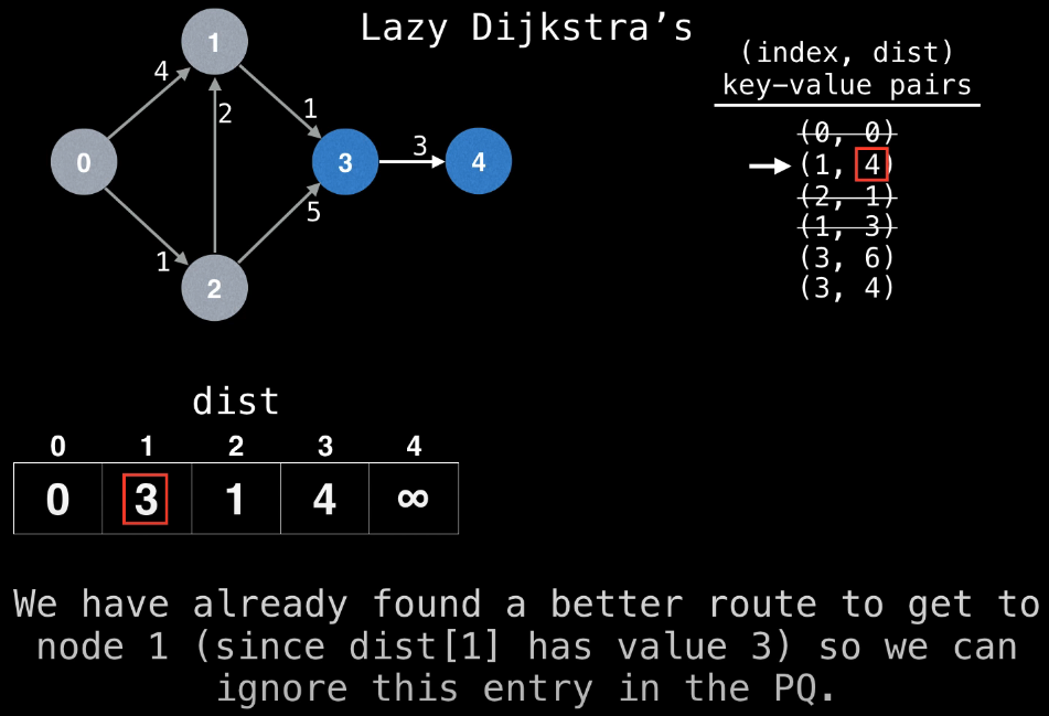
The small graph example above shows there are two ways to get from node 0 (the source node) to node 1:
0 -> 1: Distance of40 -> 2 -> 1: Distance of1 + 2 = 3
The second path is shorter even though there are more edges. Why does this matter? Because of how the priority queue is being used and maintained. Specifically, we add (0, 0) as the first element to the priority queue to indicate that we plan to visit node 0 with a best distance of 0. Then the algorithm actually starts and we look inside the priority queue for the first time and discover we should visit node 0. What nodes should we visit after visiting node 0? As with BFS and DFS, Dijkstra is a search algorithm; specifically, Dijkstra is a search algorithm for the shortest path to each node in a graph from a given source node — we conduct our search by visiting neighbors; that is, we will next want to visit either node 1 or node 2, with new best distances 4 and 1, respectively (both of these distances are significantly less than infinity!).
At this point, we've visited all the nodes from node 0. Our priority queue started with just the lone element (0, 0), which we poppped from the priority queue in order to visit all neighboring nodes to node 0. We visited nodes 1 and 2 in the process, adding (1, 4) and (2, 1) to the priority queue, respectively. We're now done visiting all neighbors of node 0 so which node should we visit next?
Dijkstra's algorithm always selects the next most promising node in the priority queue. To do this, simply poll the next best key-value pair from the priority queue, which is (2, 1) in this case because the distance 1 in (2, 1) is less than the distance 4 in (1, 4). So we pop (2, 1) from the priority queue and plan to visit the neighboring nodes to node 2, namely the nodes 1 and 3. At this point, our priority queue looks something like the following:
(0, 0)(1, 4) -> (2, 1) (1, 3) (3, 6)
The tuple (0, 0)0 has been fully processed. We've also updated the distance array for its neighboring nodes as we've added them to the priority queue. Then we popped (2, 1) from the priority queue as it was the most promising node; the indicator -> (2, 1) means node 2 is currently being processed. In the midst of processing node 2, we've added tuples (1, 3) and (3, 6) to the priority queue, and we've updated the distances array as well, which currently looks like the following:
0 1 2 3 4 # <- node index
[ 0, 3, 1, 6, inf ] # <- distances
Now node 2 has been fully processed and our priority queue looks as follows:
(0, 0)(1, 4)(2, 1)-> (1, 3) (3, 6)
This means the next most promising node is node 1. From node 1, we can visit node 3 for a cumulative distance of 4 from the source node; hence, we add (3, 4) to the priority queue, and then we mark (1, 3) as processed:
(0, 0)(1, 4)(2, 1)(1, 3)(3, 6) (3, 4)
What node is most promising in the priority queue now? It's (1, 4). But we have already found a better route to get to node 1 since distances[1] has a value of 3, which is less than 4. Hence, we can ignore this entry in the priority queue.
This example above shows exactly how we can find some initial path to a node (0 -> 1) and later on find a shorter path (0 -> 2 -> 1). Dijkstra is all about the shortest path being found to a node once that node has been extracted from the priority queue for the first time (e.g., (1, 3) was extracted from the priority queue first, and then (1, 4) was extracted and ignored).
In Dijkstra, we do not know the real shortest distance to a node until it is extracted from the priority queue, not when it is simply added to the priority queue (as illustrated in the concrete example above).
In eager Dijkstra, we update the priority (i.e., distance) of the nodes in the priority queue when we find a shorter path. In lazy Dijkstra, we simply add the node again with the new priority without removing the previous occurrence of that node in the PQ. Hence, in lazy Dijkstra, nodes can appear multiple times in the priority queue with different priorities. This is not a problem. Why? Because we only care about the first time we extract a node from the priority queue. That first time gives us the shortest distance from the source node to the node just popped from the priority queue. The second time (and any subsequent times) the same node is popped from the priority queue, we simply discard the node as soon as we extract it by means of the following lines from the template:
# ...
curr_dist, node = heapq.heappop(min_heap)
if curr_dist > distances[node]:
continue
# ...
Dijkstra with a target/destination node
If we only care about the distance or shortest path from the source to a specific node, target, then we can halt the algorithm with an early termination as soon as we extract the target node from min_heap (not as soon as we add the target node to min_heap). In Dijkstra, unlike in BFS, we only know that we have found the shortest distance to a node once we have extracted it for the first time from the priority queue, min_heap in the case of the template:
# T: O(E log V); S: O(V + E)
def dijkstra(graph, source, target):
n = len(graph) # Dijkstra on graph with n nodes
distances = [float('inf')] * n # "infinitely" far from source (unvisited nodes)
distances[source] = 0
min_heap = []
heapq.heappush(min_heap, (0, source)) # heap contents: (d(v, source), v), where
# d gives a distance from source node
# to node v, another node in graph
while min_heap:
curr_dist, node = heapq.heappop(min_heap)
if node == target:
return curr_dist
if curr_dist > distances[node]: # optimization for lazy Dijkstra: ignore current path
continue # if we already found a better one (i.e., node was previously
# extracted from min_heap with a smaller distance)
for neighbor, weight in graph[node]:
dist = curr_dist + weight
if dist < distances[neighbor]: # add neighbor to min_heap if it creates a shorter path
distances[neighbor] = dist
heapq.heappush(min_heap, (dist, neighbor))
return float('inf')
Dijkstra with shortest path reconstruction
Dijkstra finds the shortest path from a source node to all other nodes in a graph. If we want to reconstruct the shortest paths themselves, then we need to compute the predecessors of each node in the shortest path tree. A small modification to the template is needed:
# T: O(E log V); S: O(V + E)
def dijkstra(graph, source):
n = len(graph) # Dijkstra on graph with n nodes
distances = [float('inf')] * n # "infinitely" far from source (unvisited nodes)
distances[source] = 0
pred = [None] * n
min_heap = []
heapq.heappush(min_heap, (0, source)) # heap contents: (d(v, source), v), where
# d gives a distance from source node
# to node v, another node in graph
while min_heap:
curr_dist, node = heapq.heappop(min_heap)
if curr_dist > distances[node]: # optimization for lazy Dijkstra: ignore current path
continue # if we already found a better one (i.e., node was previously
# extracted from min_heap with a smaller distance)
for neighbor, weight in graph[node]:
dist = curr_dist + weight
if dist < distances[neighbor]: # add neighbor to min_heap if it creates a shorter path
distances[neighbor] = dist
pred[neighbor] = node
heapq.heappush(min_heap, (dist, neighbor))
return distances, pred
All that remains is to reverse the steps from any given node to the source and then reverse that path to get the original shortest path from source to destination.
# T: O(E log V); S: O(V + E)
def dijkstra_shortest_path(graph, source, target):
distances, predecessors = dijkstra(graph, source)
path = []
# if target node is not accessible from source node,
# then return an empty path
if distances[target] == float('inf'):
return path
# traverse the previous nodes to build the path
node = target
while node is not None:
path.append(node)
node = predecessors[node]
# reverse the path to get the correct order from start to end
path.reverse()
return path
# T: O(E log V); S: O(V + E)
def dijkstra(graph, source):
n = len(graph) # Dijkstra on graph with n nodes (assumed to be adjacency list)
distances = [float('inf')] * n # "infinitely" far from source (unvisited nodes)
distances[source] = 0
min_heap = []
heapq.heappush(min_heap, (0, source)) # heap contents: (d(v, source), v), where
# d gives a distance from source node
# to node v, another node in graph
while min_heap:
curr_dist, node = heapq.heappop(min_heap)
if curr_dist > distances[node]: # optimization for lazy Dijkstra: ignore current path
continue # if we already found a better one (i.e., node was previously
# extracted from min_heap with a smaller distance)
for neighbor, weight in graph[node]:
dist = curr_dist + weight
if dist < distances[neighbor]: # add neighbor to min_heap if it creates a shorter path
distances[neighbor] = dist
heapq.heappush(min_heap, (dist, neighbor))
return distances
Examples
LC 743. Network Delay Time (✓)
You are given a network of n nodes, labeled from 1 to n. You are also given times, a list of travel times as directed edges times[i] = (ui, vi, wi), where ui is the source node, vi is the target node, and wi is the time it takes for a signal to travel from source to target.
We will send a signal from a given node k. Return the time it takes for all the n nodes to receive the signal. If it is impossible for all the n nodes to receive the signal, return -1.
class Solution:
def networkDelayTime(self, times: List[List[int]], n: int, k: int) -> int:
def build_graph(edge_list):
graph = defaultdict(list)
for source, destination, time in edge_list:
graph[source].append((destination, time))
return graph
graph = build_graph(times)
time_cost = [float('inf')] * (n + 1)
time_cost[0] = 0
time_cost[k] = 0
min_heap = [(0, k)]
while min_heap:
curr_time, node = heapq.heappop(min_heap)
if curr_time > time_cost[node]:
continue
for neighbor, time in graph[node]:
new_time = curr_time + time
if new_time < time_cost[neighbor]:
time_cost[neighbor] = new_time
heapq.heappush(min_heap, (new_time, neighbor))
min_time = 0
for time in time_cost:
if time == float('inf'):
return -1
min_time = max(min_time, time)
return min_time
In some ways, this is sort of a quintessential Dijkstra problem. We need to minimize the path from the source node, k, to all other nodes. Since nodes are numbered 1 through n, inclusive, we pretend as if there are n + 1 nodes in order to simplify the mechanics — we subsequently set the time cost for the dummy node and source node to 0 (i.e., nodes 0 and k, respectively).
Time: TBD
Space: TBD
LC 787. Cheapest Flights Within K Stops (✓) ★★★
There are n cities connected by m flights. Each flight starts from city u and arrives at v with a price w.
Now given all the cities and flights, together with starting city src and the destination dst, your task is to find the cheapest price from src to dst with up to k stops. If there is no such route, output -1.
class Solution:
def findCheapestPrice(self, n: int, flights: List[List[int]], src: int, dst: int, k: int) -> int:
def build_graph(edges):
graph = defaultdict(list)
for start, end, cost in edges:
graph[start].append((end, cost))
return graph
graph = build_graph(flights)
cost = [[float('inf')] * (k + 2) for _ in range(n)] # cheapest cost for node by jumps
cost[src][0] = 0 # 0 cost for 0th jump to starting point
min_heap = [(0, 0, src)] # (cost, stops, node)
while min_heap:
curr_cost, curr_stops, node = heapq.heappop(min_heap)
if node == dst:
return curr_cost
if curr_stops > k:
continue
for neighbor, price in graph[node]:
new_cost = curr_cost + price
new_stops = curr_stops + 1
if new_cost < cost[neighbor][new_stops]:
cost[neighbor][new_stops] = new_cost
heapq.heappush(min_heap, (new_cost, new_stops, neighbor))
return -1
The main twist for Dijkstra in this problem is that the cheapest path to any given node may be valid or invalid based on the number of stops required to get there. We need to handle cheapest path determinations carefully. The "normal" Dijkstra algorithm would suffice if we had (i.e., if we allowed an infinite number of stops) because the problem is simply reduced to a traditional shortest path problem. But when there is a limit on the number of stops, k, the problem becomes more complex because it's not just about finding the shortest path but the shortest path within a constrained number of stops. This constraint fundamentally changes the nature of the problem (and hence the nature of our Dijkstra implementation): We can no longer simply use the shortest distance globally (i.e., just using a distances array) — we need to keep the best possible distance for each node considering the number of stops used to get there.
This means we need to use a data structure that can record both the cumulative total cost to get to a node as well as the number of stops involved. In the solution above, we use the following structure:
cost = [[float('inf')] * (k + 2) for _ in range(n)]
In the context of the flight problem, a "stop" means a node visited on the path from the source to the destination, not the act of moving from one node to another. Hence, if our path were 0 -> 1 -> 2, then there is only one "stop" even though three nodes are involved. If we have n nodes and k stops, then cost will look like
cost = [
# [ before first stop, first stop, ..., last stop, after last stop ] # node 0
# [ before first stop, first stop, ..., last stop, after last stop ] # node 1
# ...
# [ before first stop, first stop, ..., last stop, after last stop ] # node n - 1
]
where each of the n entries are k + 2 units long (with all default values equal to inf). We fill the cost array for each node, where each of the k + 2 slots indicate the minimum cost for reaching that node in that many stops. Hence, the source node will have a cost of 0 in its first slot because we begin at that point with no associated cost. The first slot for all other nodes is inf because there's no way to reach such nodes before the first stop.
For the sake of optimization, as soon as the destination node is popped from the priority queue, we should return curr_cost because this cost is guaranteed to represent the cheapest path to the destination node.
Time: TBD.
Space: TBD.
The following solution is also a viable way of approaching this problem:
class Solution:
def findCheapestPrice(self, n: int, flights: List[List[int]], src: int, dst: int, k: int) -> int:
def build_graph(edge_list):
graph = defaultdict(list)
for source, destination, price in edge_list:
graph[source].append((destination, price))
return graph
graph = build_graph(flights)
min_heap = [(0, 0, src)] # cost, stops, node
costs = {(src, 0): 0} # (node, num_stops): cost ... min cost to get to node in num_stops stops
while min_heap:
curr_cost, curr_stops, node = heapq.heappop(min_heap)
if node == dst:
return curr_cost
if curr_stops <= k:
for neighbor, price in graph[node]:
new_cost = curr_cost + price
new_stops = curr_stops + 1
if (neighbor, new_stops) not in costs or new_cost < costs[(neighbor, new_stops)]:
costs[(neighbor, new_stops)] = new_cost
heapq.heappush(min_heap, (new_cost, new_stops, neighbor))
return -1
Time: TBD
Space: TBD
LC 1514. Path with Maximum Probability★★
You are given an undirected weighted graph of n nodes (0-indexed), represented by an edge list where edges[i] = [a, b] is an undirected edge connecting the nodes a and b with a probability of success of traversing that edge succProb[i].
Given two nodes start and end, find the path with the maximum probability of success to go from start to end and return its success probability.
If there is no path from start to end, return 0. Your answer will be accepted if it differs from the correct answer by at most 10-5.
class Solution:
def maxProbability(self, n: int, edges: List[List[int]], succProb: List[float], start_node: int, end_node: int) -> float:
def build_graph(edge_list):
adj_list = defaultdict(list)
for i in range(len(edge_list)):
start, end = edge_list[i]
edge_weight = succProb[i]
adj_list[start].append((end, edge_weight))
adj_list[end].append((start, edge_weight))
return adj_list
graph = build_graph(edges)
max_prob = [0.0] * n
max_prob[start_node] = 1.0
max_heap = [(-1.0, start_node)]
while max_heap:
curr_prob, node = heapq.heappop(max_heap)
curr_prob = -curr_prob
if node == end_node:
return curr_prob
if curr_prob < max_prob[node]:
continue
for neighbor, prob in graph[node]:
new_prob = curr_prob * prob
if new_prob > max_prob[neighbor]:
max_prob[neighbor] = new_prob
heapq.heappush(max_heap, (-new_prob, neighbor))
return 0
Since Python only has a min heap, we simulate a max heap by pushing the negated version of whatever current path probability exists to the node in question onto the min heap. We simply need to be careful when handling the sign of the probability (i.e., when popping from and adding to the heap).
class Solution:
def maxProbability(self, n: int, edges: List[List[int]], succProb: List[float], start_node: int, end_node: int) -> float:
def build_graph(edge_list):
adj_list = defaultdict(list)
for i in range(len(edge_list)):
start, end = edge_list[i]
edge_weight = -math.log(succProb[i])
adj_list[start].append((end, edge_weight))
adj_list[end].append((start, edge_weight))
return adj_list
max_prob = [float('inf')] * n
max_prob[start_node] = 0
graph = build_graph(edges)
max_heap = [(0, start_node)]
while max_heap:
curr_prob, node = heapq.heappop(max_heap)
if curr_prob > max_prob[node]:
continue
for nei in graph[node]:
nei_node, path_prob = nei
new_prob = curr_prob + path_prob
if new_prob < max_prob[nei_node]:
max_prob[nei_node] = new_prob
heapq.heappush(max_heap, (new_prob, nei_node))
return math.exp(-max_prob[end_node])
The solution above uses logarithms to increase precision. It is largely based on observations highlighted in this solution comment:
I am surprised to see such a long editorial (three different algorithms with a lot of what sounds like chat GPT generated explanations of the code and a plethora of diagrams) that at no point attempts to justify why using these algorithms give the correct answer for the problem.
"We need to find the path from start to end that has the largest product of its edges" - fine
"BFS is an algorithm I know but it's not used on graphs with weighted edges, let's use Dijkstra instead because that one works on weighted graphs" - cool story bro, but Dijkstra is a shortest path algorithm, not a largest product algorithm...
For anyone who is curious why it works and hasn't worked it out themselves:
- Call product of the edges in a path
- We want to find the path with maximum .
- Since the logarithm is a monotonically growing function, the path with largest is also the path with largest , (and the smallest )
- Due to the properties of the logarithm,
- Negating both sides gives us the following: .
- In summary: maximizing , the explicit goal of the problem, is equivalent to minimizing , which is just the sum of the negative logarithms of the edge weights. This equivalent modified problem IS a shortest path problem.
- Furthermore, since , that means and . Non-negative edges, a requirement for Dijkstra to work properly.
- So yeah, TL;DR: "weighted graph, can't be BFS, let's use Dijkstra" is dumb, but since edge weights are probabilities, finding the maximum product is equivalent to a shortest path problem with non-negative edge weights, and Dijkstra "just works"
ChatGPT sheds some light on why we might want to use logarithms for certain problems:
- Problem: When calculating the product of many terms, especially in probabilities (e.g., in Bayesian inference or machine learning), the product can become extremely small, leading to underflow.
- Solution: Take the logarithm of each term, sum these logarithms, and then exponentiate the result. This approach is particularly useful in algorithms like the Viterbi algorithm or when dealing with partition functions in statistical mechanics.
The equality we take advantage of is as follows:
Bellman-Ford
Intuition for Bellman-Ford algorithm
Bellman-Ford, despite its innocent and simplistic appearance on the surface, can be rather difficult to learn at first. As a popular video on Bellman-Ford notes:
Of all the shortest path algorithms in graph theory, Bellman-Ford is definitely one of the simplest; yet, I struggled as an undergrad student trying to learn this algorithm, which is part of the reason I'm making this video.
Part of the struggle may be be rooted in how this algorithm is taught/introduced in several textbooks. It is informative to look at expositions on this algorithm in [20] (DPV) and [24] (CLRS). Specifically, we look at the introductions and examples provided in both texts, test the examples with our template, and then return to unearth a key revelation that is likely the source of struggle for many people first learning this algorithm.
Description and example in DPV
The exposition that follows is based on what appears in [20] (some parts have been modified so as to ensure these remarks are self-contained).
Dijkstra's algorithm [yes, Dijkstra's algorithm is covered before Bellman-Ford in DPV] works in part because the shortest path from the starting point to any node must pass exclusively through nodes that are closer than . This no longer holds when edge lengths can be negative. In the figure below, the shortest path from to passes through , a node that is further away! [Comically, the edge weight of is clearly an error and should instead read .]

What needs to be changed in order to accommodate this new complication? To answer this, let's take a particular high-level view of Dijkstra's algorithm. A crucial invariant is that the dist values it maintains are always either overestimates or exactly correct. They start off at , and the only way they ever change is by updating along an edge:
PROCEDURE UPDATE((u, v) in E)
dist(v) = min{dist(v), dist(u) + l(u, v)}
This update operation is simply an expression of the fact that the distance to cannot possibly be more than the distance to , plus . It has the following properties.
- It gives the correct distance to in the particular case where is the second-last node in the shortest path to , and is correctly set.
- It will never make too small, and in this sense it is safe. For instance, a slew of extraneous
update's can't hurt.
This operation is extremely useful: it is harmless, and if used carefully, will correctly set distances. In fact, Dijkstra's algorithm can be thought of simply as a sequence of update's. We know this particular sequence doesn't work with negative edges, but is there some other sequence that does? To get a sense of the properties this sequence must possess, let's pick a node and look at the shortest path to it from .

This path can have at most edges. Why? The answer is probably more nuanced than it seems at first. The following explanation is given in [24]:
Can a shortest path contain a cycle? As we have just seen, it cannot contain a negative-weight cycle. Nor can it contain a positive-weight cycle, since removing the cycle from the path produces a path with the same source and destination vertices and a lower path weight. That is, if is a path and is a positive-weight cycle on this path (so that and ), then the path has weight , and so cannot be a shortest path from to .
That leaves only 0-weight cycles. You can remove a 0-weight cycle from any path to produce another path whose weight is the same. Thus, if there is a shortest path from a source vertex to a destination vertex that contains a 0-weight cycle, then there is another shortest path from to without this cycle. As long as a shortest path has 0-weight cycles, you can repeatedly remove these cycles from the path until you have a shortest path that is cycle-free. Therefore, without loss of generality, assume that shortest paths have no cycles, that is, they are simple paths.
Since any acyclic path in a graph contains at most distinct vertices [i.e., a path passing through every vertex], it also contains at most edges. Assume, therefore, that any shortest path contains at most edges.
The last paragraph above is the key takeaway. Returning to our description of the shortest path image: the shortest path from to can have at most edges per the excerpt above. If the sequence of updates performed includes , in that order (though not necessarily consecutively), then by the first property the distance to will be correctly computed. It doesn't matter what other updates occur on these edges, or what happens in the rest of the graph, because updates are safe.
But still, if we don't know all the shortest paths beforehand, how can we be sure to update the right edges in the right order? Here is an easy solution: simply update all the edges, times! The resulting procedure is called the Bellman-Ford algorithm and is shown below in pseudocode:
PROCEDURE ShortestPaths(G, l, s)
Input: Directed graph G = (V, E)
edge lengths {l_e : e in E} with no negative cycles.
Output: For all vertices u reachable from s, dist(u) is set
to the distance from s to u
for all u in V:
dist(u) = +infty
prev(u) = nil
dist(s) = 0
repeat |V| - 1 times:
for all e in E:
update(e)
An example run of the algorithm is shown below:
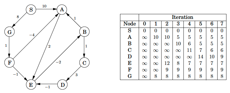
A note about implementation: for many graphs, the maximum number of edges in any shortest path is substantially less than , with the result that fewer rounds of updates are needed. Therefore, it makes sense to add an extra check to the shortest-path algorithm, to make it terminate immediately after any round in which no update occurred.
What about negative cycles? If the length of edge in the figure above were changed to , then the graph would have a negative cycle . In such situations, it doesn't make sense to even ask about shortest paths. There is a path of length 2 from to . But going round the cycle, there's also a path of length 1, and going round multiple times, we find paths of lengths 0, , , and so on.
The shortest-path problem is ill-posed in graphs with negative cycles. As might be expected, our algorithm in the pseudocode above (i.e., Bellman-Ford) works only in the absence of such cycles. But where did this assumption appear in the derivation of the algorithm? Well, it slipped in when we asserted the existence of a shortest path from to .
Fortunately, it is easy to automatically detect negative cycles and issue a warning. Such a cycle would allow us to endlessly apply rounds of update operations, reducing dist estimates every time. So instead of stopping after iterations, perform one extra round. There is a negative cycle if and only if some dist value is reduced during this final round.
Testing the DPV example with the template
To effectively test our template code, first convert the example graph into an adjacency list:
Map the letter nodes to their numeric equivalent:
S: 0
A: 1
B: 2
C: 3
D: 4
E: 5
F: 6
G: 7
Then we get the following adjacency list representation of the graph above:
graph = {
0: [(1, 10), (7, 8)],
1: [(5, 2)],
2: [(1, 1), (3, 1)],
3: [(4, 3)],
4: [(5, -1)],
5: [(2, -2)],
6: [(1, -4), (5, -1)],
7: [(6, 1)]
}
Let's now use a modified version of the template code where comments have been removed and we've added a print statement to show the distances array after each iteration of relaxing all edges:
def bellman_ford(graph, start):
n = len(graph)
distances = [float('inf')] * n
distances[start] = 0
predecessors = [None] * n
for _ in range(n - 1):
edge_updated = False
for node in range(n):
for neighbor, weight in graph[node]:
if distances[node] != float('inf') and distances[node] + weight < distances[neighbor]:
edge_updated = True
distances[neighbor] = distances[node] + weight
predecessors[neighbor] = node
print(distances)
if not edge_updated:
return distances, predecessors
for node in range(n):
for neighbor, weight in graph[node]:
if distances[node] != float('inf') and distances[node] + weight < distances[neighbor]:
return False
return distances, predecessors
graph = {
0: [(1, 10), (7, 8)],
1: [(5, 2)],
2: [(1, 1), (3, 1)],
3: [(4, 3)],
4: [(5, -1)],
5: [(2, -2)],
6: [(1, -4), (5, -1)],
7: [(6, 1)]
}
bellman_ford(graph, 0)
We get the following printed to the console (the initial distances array, before any iteration has taken place, has been included for the sake of clarity):
# S A B C D E F G
[ 0, inf, inf, inf, inf, inf, inf, inf ] # after iteration 0 (initial distances array)
[ 0, 10, 10, inf, inf, 12, 9, 8 ] # after iteration 1
[ 0, 5, 10, 11, 14, 8, 9, 8 ] # after iteration 2
[ 0, 5, 5, 11, 14, 7, 9, 8 ] # after iteration 3
[ 0, 5, 5, 6, 9, 7, 9, 8 ] # after iteration 4
[ 0, 5, 5, 6, 9, 7, 9, 8 ] # after iteration 5 (no edges updated, terminate early)
If we're first learning about Bellman-Ford, then the output above is probably very confusing. The end result, namely the final distances array, is the same as in the book's example: [0, 5, 5, 6, 9, 7, 9, 8]. But everything else (i.e., the intermediate results) is very different. Why? We'll return to this example to see why, but let's first look at the example from CLRS to get a hint.
Description and example in CLRS
The terminology and notation used in the following initial description by CLRS may be foreign, but the illustrated example should clear up any confusion.
The Bellman-Ford algorithm solves the single-source shortest-paths problem in the general case in which edge weights may be negative. Given a weighted, directed graph with source vertex and weight function , the Bellman-Ford algorithm returns a boolean value indicating whether there is a negative-weight cycle that is reachable from the source. If there is such a cycle, the algorithm indicates that no solution exists. If there is no such cycle, the algorithm produces the shortest paths and their weights.
The procedure BELLMAN-FORD relaxes edges, progressively decreasing an estimate on the weight of a shortest path from the source to each vertex until it achieves the actual shortest-path weight . The algorithm returns TRUE if and only if the graph contains no negative-weight cycles that are reachable from the source.
% page 612 (CLRS 4th Ed.)
\begin{algorithm}
\caption{\textsc{Bellman-Ford}($G, w, s$)}
\begin{algorithmic}
\PROCEDURE{Initialize-Single-Source}{$G, s$}\ENDPROCEDURE
\FOR{$i=1$ to $|G.v| - 1$}
\FOR{each edge $(u, v)\in G.E$}
\PROCEDURE{RELAX}{$u, v, w$}\ENDPROCEDURE
\ENDFOR
\ENDFOR
\FOR{each edge $(u, v)\in G.E$}
\IF{$v.d > u.d + w(u, v)$}
\RETURN \textsc{false}
\ENDIF
\ENDFOR
\RETURN \textsc{true}
\end{algorithmic}
\end{algorithm}The figure below shows the execution of the Bellman-Ford algorithm on a graph with 5 vertices. After initializing the and values of all vertices in line 1, the algorithm makes passes over the edges of the graph. Each pass is one iteration of the for loop of lines 2-4 and consists of relaxing each edge of the graph once. Figures (b)-(e) show the state of the algorithm after each of the four passes over the edges. After making passes, lines 5-8 check for a negative-weight cycle and return the appropriate boolean value.
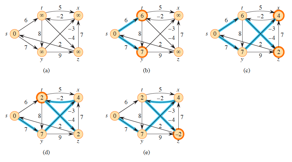
The figure above shows the execution of the Bellman-Ford algorithm. The source is vertex . The values appear within the vertices, and blue edges indicate predecessor values: if edge is blue, then . In this particular example, each pass relaxes the edges in the order , , , , , , , , , . (a) The situation just before the first pass over the edges. (b)–(e) The situation after each successive pass over the edges. Vertices whose shortest-path estimates and predecessors have changed due to a pass are highlighted in orange. The and values in part (e) are the ûnal values. The Bellman-Ford algorithm returns TRUE in this example.
Testing the CLRS example with the template
Let's see if we can test our template against the example provided in CLRS:
As with the DPV example, we should start by mapping the letter nodes to their numeric equivalent. What number should we assign to each node? The order in which each edge is relaxed suggests a natural labeling scheme:
[
(t, x), (t, y), (t, z), # t: 0
(x, t), # x: 1
(y, x), (y, z), # y: 2
(z, x), (z, s), # z: 3
(s, t), (s, y) # s: 4
]
What will we get when we represent the graph as an adjacency list and use the modified template as before (where we printed the distances array after each iteration)? Let's see:
def bellman_ford(graph, start):
# ...
graph = {
0: [(1, 5), (2, 8), (3, -4)],
1: [(0, -2)],
2: [(1, -3), (3, 9)],
3: [(1, 7), (4, 2)],
4: [(0, 6), (2, 7)],
}
bellman_ford(graph, 4)
We get the following printed to the console (the initial distances array, before any iteration has taken place, has been included for the sake of clarity):
# t x y z s
[ inf, inf, inf, inf, 0 ] # after iteration 0 (initial distances array)
[ 6, inf, 7, inf, 0 ] # after iteration 1
[ 6, 4, 7, 2, 0 ] # after iteration 2
[ 2, 4, 7, 2, 0 ] # after iteration 3
[ 2, 4, 7, -2, 0 ] # after iteration 4 (|V| - 1 iterations with no negative cycle)
Each line above exactly matches the figures (a)-(e), respectively. How is it possible that our template reproduced exactly what was given in CLRS and was not even close for DPV? The key revelation is provided in the next and final remark.
Key revelation via basic example: order of edge relaxation does not effect end result but completely determines intermediate results
As another comment mentions in the previously linked video, let's consider the very basic linearly connected graph 0 -> 1 -> 2 -> 3, where the source node is 0 and all edge weights are 1. Such a graph may be represented in code with the following adjacency list:
graph = {
0: [(1, 1)],
1: [(2, 1)],
2: [(3, 1)],
3: []
}
Since the order of edge updates in Bellman-Ford is random, let's consider what would happen in the worst possible case. For the first iteration, we would update the edge 0 -> 1 at the end; that is, let's purposely let the edge 0 -> 1 be the last edge we "randomly" update. For the graph 0 -> 1 -> 2 -> 3 with edge weights 1, this means 0 -> 1 is the only edge whose relaxation/processing reduces the distances to a node (i.e., the distance to node 1 is now 1 instead of infinity). Similarly, for iterations 2 and 3 we update 1 -> 2 and 2 -> 3 at the end:
[0, inf, inf, inf] # after iteration 0 (initial distances array)
[0, 1, inf, inf] # after iteration 1
[0, 1, 2, inf] # after iteration 2
[0, 1, 2, 3] # after iteration 3 (|V| - 1 iterations with no negative cycle)
Hence, in the worst case, it can take iterations to propagate the edge weights appropriately. Let's test our template code with this basic graph. If we run the same template code that we ran for the examples in DPV and CLRS, then we get the following:
[0, inf, inf, inf] # after iteration 0 (initial distances array)
[0, 1 2, 3] # after iteration 1
[0, 1 2, 3] # after iteration 2 (no edges updated, terminate early)
What's going on? Why aren't we getting the results discussed above? Because the results discussed above were in the worst case, where we purposely delayed processing the edge connected to the source node until the end. Let's examine the template code:
def bellman_ford(graph, start):
n = len(graph)
distances = [float('inf')] * n
distances[start] = 0
predecessors = [None] * n
for _ in range(n - 1):
edge_updated = False
for node in range(n):
for neighbor, weight in graph[node]:
if distances[node] != float('inf') and distances[node] + weight < distances[neighbor]:
edge_updated = True
distances[neighbor] = distances[node] + weight
predecessors[neighbor] = node
print(distances)
if not edge_updated:
return distances, predecessors
for node in range(n):
for neighbor, weight in graph[node]:
if distances[node] != float('inf') and distances[node] + weight < distances[neighbor]:
return False
return distances, predecessors
The highlighted line for node in range(n): ensures we always start edge relaxations from the node with label 0, whether or not that node is the source node. Recall the edge labeling from the CLRS example:
[
(t, x), (t, y), (t, z), # t: 0
(x, t), # x: 1
(y, x), (y, z), # y: 2
(z, x), (z, s), # z: 3
(s, t), (s, y) # s: 4
]
Note how the source node, highlighted above, has a node label of 4. This means that all edges connected to the source update at the end when for node in range(n): fires. Hence, the only edges relaxed in a meaningful way after the first iteration are those directly connected with the source node.
What if we changed the highlighted line for node in range(n): to for node in [3, 2, 1, 0]: for the basic graph example? Then all edges directly connected to the source node are processed last. We're basically customizing our template to be as inefficient as possible so as to show how we can ensure the maximum number of iterations occur. And, sure enough, running the template code with this modification results in exactly what we discussed for the worst case scenario:
[0, inf, inf, inf] # after iteration 0 (initial distances array)
[0, 1, inf, inf] # after iteration 1
[0, 1, 2, inf] # after iteration 2
[0, 1, 2, 3] # after iteration 3 (|V| - 1 iterations with no negative cycle)
Using the key revelation to better understand the DPV example
Let's return to the DPV example that started all of this:
Running our template code resulted in the following:
# S A B C D E F G
[ 0, inf, inf, inf, inf, inf, inf, inf ] # after iteration 0 (initial distances array)
[ 0, 10, 10, inf, inf, 12, 9, 8 ] # after iteration 1
[ 0, 5, 10, 11, 14, 8, 9, 8 ] # after iteration 2
[ 0, 5, 5, 11, 14, 7, 9, 8 ] # after iteration 3
[ 0, 5, 5, 6, 9, 7, 9, 8 ] # after iteration 4
[ 0, 5, 5, 6, 9, 7, 9, 8 ] # after iteration 5 (no edges updated, terminate early)
The end result was the same as that in the figure, but the intermediate results were very different. The "key revelation" discussion in the previous widget explains why. The line for node in range(n): in the main loop of our template code ensured we started by processing all edges directly connected to whatever node was labelled 0. Of course, in this case, node S, the source node, was labelled as node 0, which means all edges directly connected to the source node were the first ones to be meaningfully relaxed. This efficiency would usually be considered a good thing. But not when we're trying to better understand an example!
CLRS gave us the exact order in which edges were processed, making it clear they were trying to be as inefficient as possible in order to highlight when iterations could be necessary. Similarly, if we intentionally process the edges connected to the source node last, then maybe we can go about reproducing the table provided in DPV, where iterations are necessary to get the final distances array.
After some tinkering, we discover that if we replace the line for node in range(n): in the main loop with for node in [4, 3, 2, 5, 1, 6, 7, 0]:, then we end up reproducing the table of results provided in the DPV example:
# S A B C D E F G
[ 0, inf, inf, inf, inf, inf, inf, inf ] # after iteration 0 (initial distances array)
[ 0, 10, inf, inf, inf, inf, inf, 8 ] # after iteration 1
[ 0, 10, inf, inf, inf, 12, 9, 8 ] # after iteration 2
[ 0, 5, 10, inf, inf, 8, 9, 8 ] # after iteration 3
[ 0, 5, 6, 11, inf, 7, 9, 8 ] # after iteration 4
[ 0, 5, 5, 7, 14, 7, 9, 8 ] # after iteration 5
[ 0, 5, 5, 6, 10, 7, 9, 8 ] # after iteration 6
[ 0, 5, 5, 6, 9, 7, 9, 8 ] # after iteration 7 (|V| - 1 iterations with no negative cycle)
What's the exact order in which the edges were processed? Since the letter-number mapping for the nodes in this example is
D, C, B, E, A, F, G, S
[4, 3, 2, 5, 1, 6, 7, 0]
we can use the adjacency list representation of the graph
graph = {
0: [(1, 10), (7, 8)],
1: [(5, 2)],
2: [(1, 1), (3, 1)],
3: [(4, 3)],
4: [(5, -1)],
5: [(2, -2)],
6: [(1, -4), (5, -1)],
7: [(6, 1)]
}
to fully specify the order in which edges are relaxed for each iteration:
# D, C, B, E, A, F, G, S
# [4, 3, 2, 5, 1, 6, 7, 0]
[
(D, E), # D-connected edges
(C, D), # C-connected edges
(B, A), (B, C), # B-connected edges
(E, B), # E-connected edges
(A, E), # A-connected edges
(F, A), (F, E), # F-connected edges
(G, F), # G-connected edges
(S, A), (S, G) # S-connected edges
]
As has been thoroughly demonstrated by now, the order in which edges are processed does not matter in terms of the end result, but the order completely determines the intermediate results of the distances array.
Why we do |V| - 1 iterations in Bellman-Ford
One of the better explanations for why exactly we do iterations in the Bellman-Ford algorithm is given in a comment, by user nmamano, on William Fiset's Bellman-Ford YouTube video, paraphrased and cleaned up a bit below.
To elaborate on why we do iterations, it comes from the following lemma:
If the shortest path from the source node to a node ends with the edge , and we already know the correct distance to (i.e., shortest distance from the source node to node ), and then we relax the edge , then we will find the correct distance to .
It may seem like a pretty obvious lemma, but the correctness of Bellman-Ford, Dijkstra, and topological sort are all based on it:
- Dijkstra's Algorithm: Utilizes this lemma by always selecting the unvisited node with the smallest known distance (the "greedy" approach), ensuring that when an edge is relaxed, the distance to is already optimal. (This is why each edge only needs to be relaxed once.)
- Topological Sort-Based Algorithms: In Directed Acyclic Graphs (DAGs), nodes are processed in a topological order, guaranteeing that when processing node , all predecessors have been processed, and their distances are correct. (This is why each edge only needs to be relaxed once.)
- Bellman-Ford Algorithm: Cannot rely on a specific processing order due to the presence of cycles and negative edge weights. It compensates by repeatedly relaxing all edges, ensuring that the correct distances eventually propagate through the graph.
The consequence of this lemma is that, in order to find the correct distance to a node , we need to relax all the edges in the shortest path from the source to IN ORDER.
Dijkstra and topological sort are efficient because we only relax the out-going edges from each node after we found the correct distance for that node, so we only need to relax the edges once. Unfortunately, the combination of cycles and negative edges makes it impossible to find a "good" order to relax the edges. Thus, Bellman-Ford just relaxes all the edges in an arbitrary order (this is one iteration of Bellman-Ford).
- In the first iteration, we find the correct distance for all the nodes whose shortest paths from the source have 1 edge.
- In the next iteration, we find the correct distances for all the nodes whose shortest paths from the source have 2 edges, and so on.
- If the shortest path with the most edges has edges, then we need iterations of Bellman-Ford. Of course, we do not know what is in advance, but, since shortest paths never repeat nodes (assuming there are no negative cycles), then what we know for sure is that any shortest path will have at most edges (in the case where it goes through every node).
This is why iterations is ALWAYS enough (but often not necessary). If in one iteration of Bellman-Ford no relaxation yields any improvement, then it means that we already found all shortest paths and we can finish.
Bellman-Ford with shortest path reconstruction
Bellman-Ford finds the shortest path from a source node to all other nodes in a graph unless there is a negative cycle. Hence, if running the Bellman-Ford algorithm in the template returns False, then no shortest path from a source node to a target node may be found; otherwise, the process for determining the shortest path is virtually the same as that used with Dijkstra:
# T: O(VE); S: O(V + E)
def bellman_ford_shortest_path(graph, source, target):
res = bellman_ford(graph, source)
if not res:
return []
distances, predecessors = res
path = []
if distances[target] == float('inf'):
return path
node = target
while node is not None:
path.append(node)
node = predecessors[node]
path.reverse()
return path
Bellman-Ford to get shortest paths despite negative cycles
Bellman-Ford is an SSSP algorithm, which means it will find the shortest path from a source node to all other nodes in the graph. Unless there is a negative-weight cycle! Then it's possible for paths to exist that can be made infinitely negative by virtue of the negative cycle. Specifically, shortest paths cannot exist for nodes that either lie directly on a negative-weight cycle or are reachable by a negative-weight cycle.
Is our shortest path work useless if a negative cycle exists or can we salvage it by still finding shortest paths to the nodes that are neither on nor reachable from a negative-weight cycle? We can salvage it! As this video notes, we basically need to iterate over all edges again, marking nodes on or reachable from negative-weight cycles by to indicate a weight of negative infinity and updating their predecessor values to None. How many times do we need to iterate over all edges again? A maximum of times in order to let the negatively infinite values fully propagate throughout the graph:
# T: O(VE); S: O(V + E)
def bellman_ford(graph, start):
n = len(graph) # graph assumed to be an adjacency list of n nodes
distances = [float('inf')] * n
distances[start] = 0
predecessors = [None] * n
# main loop: run |V| - 1 times (i.e., n - 1 times)
for _ in range(n - 1):
# optimization: return early if no edge is updated after relaxing all edges
edge_updated = False
# relax every edge in the graph
for node in range(n):
for neighbor, weight in graph[node]:
if distances[node] != float('inf') and distances[node] + weight < distances[neighbor]:
edge_updated = True
distances[neighbor] = distances[node] + weight
predecessors[neighbor] = node
if not edge_updated:
return distances, predecessors
# run main loop again for negative cycle detection
# if negative cycle exists, then update nodes
# on the cycle or reachable by the cycle to have a
# weight of -infinity
# run a maximum of |V| - 1 times to ensure -infinity
# values propagate throughout the entire graph
for _ in range(n - 1):
edge_updated = False
for node in range(n):
for neighbor, weight in graph[node]:
if distances[node] != float('inf') and distances[node] + weight < distances[neighbor]:
edge_updated = True
distances[neighbor] = float('-inf')
predecessors[neighbor] = None
if not edge_updated:
return distances, predecessors
return distances, predecessors
Now consider the example graph from the video:
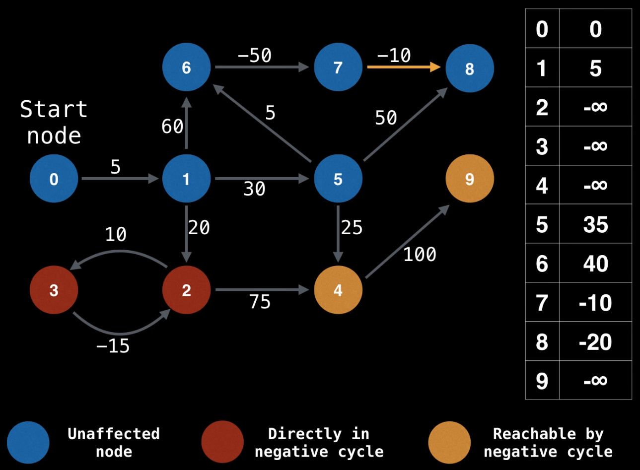
Let's try out our code on this graph:
graph = {
0: [(1, 5)],
1: [(2, 20), (5, 30), (6, 60)],
2: [(3, 10), (4, 75)],
3: [(2, -15)],
4: [(9, 100)],
5: [(4, 25), (6, 5), (8, 50)],
6: [(7, -50)],
7: [(8, -10)],
8: [],
9: [],
}
def bellman_ford(graph, start):
# ...
bellman_ford(graph, 0) # Output:
# Distances: [0, 5, -inf, -inf, -inf, 35, 40, -10, -20, -inf]
# Predecessors: [None, 0, None, None, None, 1, 5, 6, 7, None]
The result above confirms the graphic from the video. It looks like we should still be able to determine the shortest path from node 0 to node 6 though (using the shortest path reconstruction code from a previous remark):
bellman_ford_shortest_path(graph, 0, 6)
# Output: [0, 1, 5, 6]
This also confirms what we can see in the graphic from the video.
Bellman-Ford with reconstructed negative cycle
If a negative cycle exists, then we can modify our Bellman-Ford template to capture and return the first negative cycle we discover (the highlighted code below has been added to the template):
# T: O(VE); S: O(V + E)
def bellman_ford(graph, start):
n = len(graph) # graph assumed to be an adjacency list of n nodes
distances = [float('inf')] * n
distances[start] = 0
predecessors = [None] * n
# main loop: run |V| - 1 times (i.e., n - 1 times)
for _ in range(n - 1):
# optimization: return early if no edge is updated after relaxing all edges
edge_updated = False
# relax every edge in the graph
for node in range(n):
for neighbor, weight in graph[node]:
if distances[node] != float('inf') and distances[node] + weight < distances[neighbor]:
edge_updated = True
distances[neighbor] = distances[node] + weight
predecessors[neighbor] = node
if not edge_updated:
return distances, predecessors
# run main loop 1 more time for negative cycle detection
# (return a negative cycle if it exists)
for node in range(n):
for neighbor, weight in graph[node]:
if distances[node] != float('inf') and distances[node] + weight < distances[neighbor]:
curr = neighbor # negative cycle exists (start exploring predecessor chain from neighbor node)
visited = set() # keep track of which nodes have been visited
while curr not in visited:
visited.add(curr)
curr = predecessors[curr]
if curr in visited: # if node X has already been visited, then we can start cycle construction with node X
negative_cycle = [curr]
cycle_node = predecessors[curr] # explore the predecessor value chain for X
while cycle_node != negative_cycle[0]: # until we encounter X again, closing the cycle
negative_cycle.append(cycle_node) # append nodes to cycle as encountered
cycle_node = predecessors[cycle_node]
negative_cycle.reverse() # reverse cycle construction to get actual path
return negative_cycle
return distances, predecessors
The highlighted portion of the code above effectively answers the following exercise from [24]:
Suppose that a weighted, directed graph contains a negative-weight cycle. Give an efficient algorithm to list the vertices of one such cycle. Prove that your algorithm is correct.
Note that we are trying to find the vertices for any negative-weight cycle. We are not trying to enumerate them all or even find a specific one (e.g., the most negative cycle). There could be exponentially many negative cycles, and it's not in our interest to try to find them all. We will usually be satisfied with an existential determination about negative-weighted cycles: Does one exist?
- No? Great, then we can fully describe the shortest path from the source node to all other nodes!
- Yes? Uh-oh. Then that means the shortest path to all other nodes does not exist. We might be able to find the shortest path from the source to nodes not reachable by any negative cycles, but the main use case for the algorithm fails.
What if an existential determination (like the ones above) is not enough? What if we're actually interested in finding the vertices themselves that make up a negative-weighted cycle? Then we can go back up the predecessor chain to find the cycle. Specifically, we go back through the edges one more time after the main loop (i.e., where we normally do a simple negative cycle check and then call it a day).
Once we find an edge (node, neighbor) for which distances[node] + weight < distances[neighbor], then we know that either vertex neighbor is on a negative-weight cycle or is reachable from one. We can find a vertex on the negative weight-cycle by tracing back the predecessor values from neighbor, keeping track of which vertices we've visited until we reach a vertex X that we've visited before. Then we can trace back predecessor values from X until we get back to X, and all vertices in between, along with X, will constitute a negative-weight cycle.
In the code above, if the condition if curr in visited: fires after the assignment curr = predecessors[curr], then we will know that we have seen curr before (the role of X in the explanation above) and we can use curr and its predecessor values to reconstruct whatever negative-weight cycle we have just discovered, ending when cycle_node == negative_cycle[0] because that means we have traced back the predecessor values of curr until we have reached curr again. The last step is to reverse the ordering of the negative-weighted cycle nodes we've been recording because we want the returned list to represent the actual path of the negative-weight cycle.
A couple examples may help solidify the use of the code above (the first two examples reference [20] while the last example is from William Fiset's YouTube series).
Examples
Recall the graph from [20] (skip to the third example for a different self-contained example):
Everything is easier if we map the nodes to their numeric equivalent as in the table to the right of the graph above:
S: 0
A: 1
B: 2
C: 3
D: 4
E: 5
F: 6
G: 7
Once we do this, we can represent the pictured graph as an adjacency list in code as follows:
graph = {
0: [(1, 10), (7, 8)],
1: [(5, 2)],
2: [(1, 1), (3, 1)],
3: [(4, 3)],
4: [(5, -1)],
5: [(2, -2)],
6: [(1, -4), (5, -1)],
7: [(6, 1)]
}
Now let's consider two examples where negative cycles are introduced.
Example 1
As the authors note, if the length of the edge is changed to , then the graph would have a negative cycle , which we can represent as a collection of nodes (with numerical mapping): [1, 5, 2]. Let's run our code on this new graph and see what we get:
def bellman_ford(graph, start):
# ...
graph = {
0: [(1, 10), (7, 8)],
1: [(5, 2)],
2: [(1, 1), (3, 1)],
3: [(4, 3)],
4: [(5, -1)],
5: [(2, -4)],
6: [(1, -4), (5, -1)],
7: [(6, 1)]
}
bellman_ford(graph, 0) # Output: [3, 4, 5, 2]
# [C, D, E, B]
Why didn't we get [1, 5, 2]? If we look at the graph again, then we'll see that is also a negative-weight cycle when the length of the edge is changed to . Our algorithm does not discriminate between negative-weight cycles. It simply returns the first one it finds, which, in this case, happens to be .
Example 2
The example above showed how our code returns a negative-weight cycle where the source node was not involved. Is it possible for the source node to be involved? What if we negated and changed the direction of the edge so that we had the directed edge with a weight of ? Let's see:
def bellman_ford(graph, start):
# ...
graph = {
0: [(7, 8)],
1: [(0, -10), (5, 2)],
2: [(1, 1), (3, 1)],
3: [(4, 3)],
4: [(5, -1)],
5: [(2, -2)],
6: [(1, -4), (5, -1)],
7: [(6, 1)]
}
bellman_ford(graph, 0) # Output: [0, 7, 6, 1]
# [S, G, F, A]
This matches the negative-weight cycle we can see from the graph (after negating and flipping the edge): .
Example 3
The following graph is used in a video by William Fiset:
It's clear nodes 2 and 3 are the nodes directly on a negative-weighted cycle. Let's see what our code returns:
def bellman_ford(graph, start):
# ...
graph = {
0: [(1, 5)],
1: [(2, 20), (5, 30), (6, 60)],
2: [(3, 10), (4, 75)],
3: [(2, -15)],
4: [(9, 100)],
5: [(4, 25), (6, 5), (8, 50)],
6: [(7, -50)],
7: [(8, -10)],
8: [],
9: [],
}
bellman_ford(graph, 0) # Output: [2, 3]
The output indicates a negative-weighted cycle exists with path , as expected.
More interesting examples may be helpful to consider, but the examples given above should be good starting points (ha).
# T: O(VE); S: O(V + E)
def bellman_ford(graph, start):
n = len(graph) # graph assumed to be an adjacency list of n nodes
distances = [float('inf')] * n
distances[start] = 0
predecessors = [None] * n
# main loop: run |V| - 1 times (i.e., n - 1 times)
for _ in range(n - 1):
# optimization: return early if no edge is updated after relaxing all edges
edge_updated = False
# relax every edge in the graph
for node in range(n):
for neighbor, weight in graph[node]:
if distances[node] != float('inf') and distances[node] + weight < distances[neighbor]:
edge_updated = True
distances[neighbor] = distances[node] + weight
predecessors[neighbor] = node
if not edge_updated:
return distances, predecessors
# run main loop 1 more time for negative cycle detection
for node in range(n):
for neighbor, weight in graph[node]:
if distances[node] != float('inf') and distances[node] + weight < distances[neighbor]:
return False
return distances, predecessors
Examples
TBD
Prim (lazy)
Why MST algorithms work: the cut property
Before stating the cut property and working out an example or two of how that property is crucial for finding minimum spanning trees (MSTs), we should start by providing two definitions, namely what MSTs and "cuts" actually are.
First, a more formal MST definition from [20]:
MST Definition
Input: An undirected graph ; edge weights .
Output: A tree , with , that minimizes .
Second, a cut definition from Wiki:
Cut Definition
In graph theory, a cut is a partition of the vertices of a graph into two disjoint subsets. Any cut determines a cut-set, the set of edges that have one endpoint in each subset of the partition. These edges are said to cross the cut. In a connected graph, each cut-set determines a unique cut, and in some cases cuts are identified with their cut-sets rather than with their vertex partitions.
More formally, a cut is a partition of of a graph into two subsets and . The cut-set of a cut is the set of edges that have one endpoint in and the other endpoint in . If and are specified vertices of the graph , then an – cut is a cut in which belongs to the set and belongs to the set .
Note: If is partitioned into two disjoint subsets, then if is one subset, then must be the other subset. For this reason, it is common to see the set referred to above as since .
Now we can effectively state the cut property. The Wiki statement and subsequent succinct proof are quite nice:
Cut Property
For any cut of the graph, if the weight of an edge in the cut-set of is strictly smaller than the weights of all other edges of the cut-set of , then this edge belongs to all MSTs of the graph.
Proof: Assume that there is an MST that does not contain . Adding to will produce a cycle, that crosses the cut once at and crosses back at another edge . Deleting we get a spanning tree of strictly smaller weight than . This contradicts the assumption that was a MST.
By a similar argument, if more than one edge is of minimum weight across a cut, then each such edge is contained in some minimum spanning tree.
A slightly different (but also) useful statement of the cut property is given in [20]:
Suppose edges are part of a minimum spanning tree of . Pick any subset of nodes for which does not cross between and , and let be the lightest edge across this partition. Then is part of some MST.
With all of the necessary terminology in place, it may be fruitful to first consider a couple "cut" examples before remarking on why the cut property is the foundation of most MST algorithms.
Example 1
Consider the following graph:
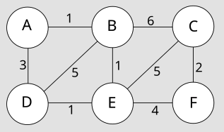
Now consider what happens when we make the following cut:
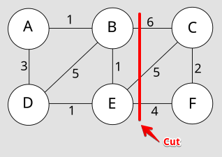
We can immediately observe a few consequences:
- Disjoint subsets: has been partitioned into two disjoint subsets: and .
- Cut set: The cut set induced by the cut is the set of edges .
- Cut property: The cut property tells us that the lightest edge in the cut set must either be in
- all MSTs if is strictly less than all other edges in the cut set or
- some MST if is not strictly less than all other edges in the cut set
For the example graph above, the edges in the cut set have weights , , and , respectively. Since weighs strictly less than all other edges in the cut set, then must be in all MSTs of the graph (there's just a single MST for the graph in this case).
Example 2
Consider the following graph:
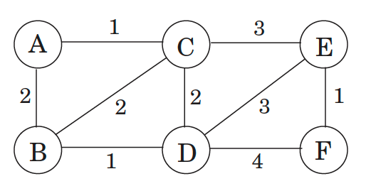
Now consider what happens when we make the following cut:
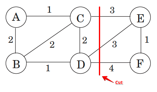
We can immediately observe a few consequences:
- Disjoint subsets: has been partitioned into two disjoint subsets: and .
- Cut set: The cut set induced by the cut is the set of edges .
- Cut property: The cut property tells us that the lightest edge in the cut set must either be in
- all MSTs if is strictly less than all other edges in the cut set or
- some MST if is not strictly less than all other edges in the cut set
For the example graph above, the edges in the cut set have weights , , and , respectively. Since and both weigh the lightest, this means each edge must be in some MST. We can see this if we produce the MSTs themselves:
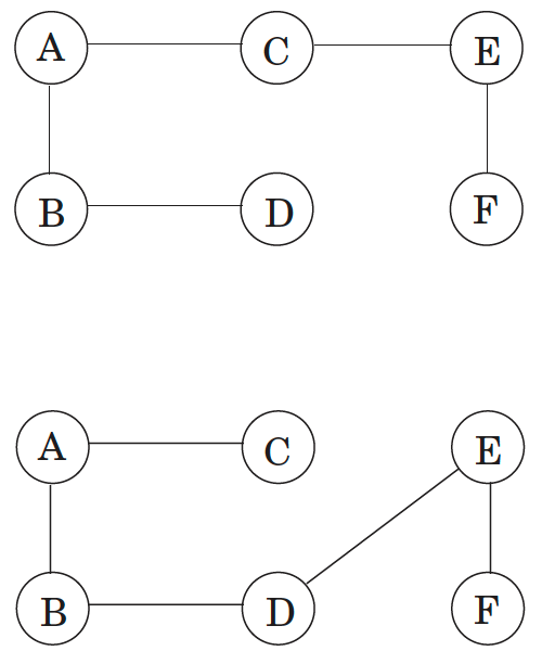
In the most general of terms, the cut property tells us that any algorithm conforming to the following greedy schema is guaranteed to work in regards to producing an MST (notated in the snippet below):
X = { } (edges picked so far)
repeat until |X| = |V| - 1:
pick a set S ⊂ V for which X has no edges between S and V − S
let e ∈ E be the minimum-weight edge between S and V − S
X = X ∪ {e}
All of the well-known MST algorithms rely on the cut property in one way or another. They simply differ in how they use this property to produce an MST:
- Prim's algorithm: Builds the MST by starting from an arbitrary vertex and repeatedly adding the smallest edge that connects a vertex in the growing MST to a vertex outside it. (Data structure: usually a min heap)
- Kruskal's algorithm: Kruskal's algorithm constructs the MST by sorting all edges and adding them one by one, ensuring that no cycles are formed. (Data structure: union-find)
- Borůvka's algorithm: Borůvka's algorithm builds the MST by repeatedly finding and adding the minimum-weight outgoing edge from each tree in the forest, effectively merging trees in phases. (Data structure: sometimes union-find but also simple structures like arrays and edge lists)
Mechanical overview of Prim's algorithm and similarity to Dijkstra
First recall the general greedy schema used by any MST algorithm:
X = { } (edges picked so far)
repeat until |X| = |V| - 1:
pick a set S ⊂ V for which X has no edges between S and V − S
let e ∈ E be the minimum-weight edge between S and V − S
X = X ∪ {e}
Prim's algorithm is probably the most popular algorithm for finding MSTs because of its intuitive nature, where, as noted in [20], the intermediate set of edges always forms a subtree, and the set is chosen to be the set of this tree's vertices.
On each iteration, the subtree defined by grows by one edge, namely the lightest edge between a vertex and a vertex outside (the edges form a tree, and consists of its vertices):
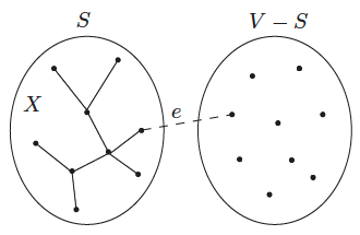
We can equivalently think of as growing to include the vertex of smallest cost:
This is strongly reminiscent of Dijkstra's algorithm. In fact the pseudocode is almost identical. The only difference is in the key values by which the priority queue is ordered:
- In Prim's algorithm, the value of a node is the weight of the lightest incoming edge from set
- In Dijkstra's algorithm, the value of a node is the length of an entire path to that node from the starting point.
Nonetheless, the two algorithms are similar enough that they have the same running time, which depends on the particular priority queue implementation. It's worth noting that the final MST produced by Prim's algorithm is completely specified by the predecessors array.
Template discussion (key components and their roles)
It's worth taking a moment to identify the key components of the template as well as what roles they play:
dist: Maintains the minimal edge weights to reach each node from the MST (which is being recorded inpred). It is essential for deciding which edge to select next.pred: Records the parent of each node in the MST. It also enables the reconstruction of the MST tree itself.visited: Ensures nodes are only included once in the MST, preventing cycles.min_heap: A priority queue that efficiently selects the next node to include based on the minimal edge weight. Note that by allowing duplicates in themin_heapand checkingvis[node]upon popping, the template avoids the complexity of updating priorities within the heap when a shorter path is found (this would require an indexed priority queue, which most languages don't support out of the box). This "lazy" approach simplifies the code and leverages the heap's properties for correctness.
Note that each vertex nbr added to the heap must have a predecessor (the only exception is whatever node we choose to be the root of our MST, the start node, which has no predecessor), specifically node, which was popped from the heap previously. When w < dist[nbr] and nbr has not yet been visited, the subsequent assignments basically amount to strategizing how to properly expand the MST we're building:
dist[nbr] = wmeans that edgenode -> nbrhas weightw, wherewis currently the best known distance from a node in the MST (i.e., currentlynode) to the nodenbroutside the MST. Of course, at some point, ifnbrhas not yet been added to the MST, then we may come acrossanother_nodein the MST that has a better distance tonbroutside the MST, in which case we would end up making the updatedist[nbr] = w_2, wherew_2is the weight of the edgeanother_node -> nbr.pred[nbr] = nodeis simply a way of ensuring that the edgenode -> nbris recorded as part of the MST if it ultimately gets added. As noted above, ifnbrhas not yet been added to the MST, and we come acrossanother_nodein the MST that has a better distance tonbroutside the MST, then the previous assignment ofpred[nbr] = nodeis overwritten by the assignmentpred[nbr] = another_node. Of course, ifanother_nodedoes not have a better distance tonbr, then we simply ignore it.
For example, consider a partial MST and a node node not yet included:
Current MST Nodes: {A, B, C}
Edges in MST: (A-B), (B-C)
Unvisited Node: D
Possible Edges: (C-D) with weight 2, (B-D) with weight 3, (A-D) with weight 1
- Edge Selection:
- When processing neighbors of
C, we find that edge(C-D)with weight2is less thandist[D](initiallyinf), so we updatedist[D] = 2andpred[D] = C. - Edge
(B-D)with weight3is not less than the currentdist[D], so we ignore it. - Edge
(A-D)with weight1is better than the currentdist[D], so we updatedist[D].
- When processing neighbors of
- Heap Insertion:
- We push
(2, D)onto themin_heap. - We push
(1, D)onto themin_heap.
- We push
- Popping from Heap:
- When
(1, D)is popped,visited[D]isFalse, so we markDas visited. - When
(2, D)is eventually popped,visited[D]isTrue, so we ignore this stale heap entry to avoid creating a cycle.
- When
- Adding Edge to MST:
- The edge from
pred[D]toDis initially(C-D), butDhas not yet been marked visited (hence the edge is not final in the MST). - The edge from
pred[D]toDis ultimately updated to be(A-D), andDis marked as visited, which means this edge is final in the MST.
- The edge from
Note how the pred array changes over time but progressively becomes fixed as nodes are added to the MST. In the example above, we started with pred[D] = None, then pred[D] = C, and finally pred[D] = A. The value pred[D] only became fixed once D was marked as visited.
Essentially, when an unvisited node is popped from the heap, we are guaranteed to add an edge to the MST (the only exception being the start node). The edge added is (pred[node], node), which connects the newly included node to the MST via the minimal edge found. This ensures the MST remains connected and includes minimal edges without forming cycles.
Time and space complexity
Time: . The algorithm's performance is dominated by heap operations, each taking time, and there are at most such operations.
Space: . Space is used to store the graph, arrays for node data, and the min-heap, all of which are bounded by .
# T: O(E log V); S: O(V + E)
def prim(graph, start = 0):
n = len(graph) # n-node graph assumed to be an adjacency list
dist = [float('inf')] * n # infinite distance for each node upon initialization
dist[start] = 0 # start can be any node, defaults to 0th node
pred = [None] * n # predecessors are marked as non-existant upon initialization
visited = [False] * n # no node has been visited upon initialization
min_heap = [] # use min heap to exploit cut property effectively
heapq.heappush(min_heap, (0, start)) # node value: weight of incoming edge from intermediate MST
while min_heap:
_, node = heapq.heappop(min_heap) # only the node itself is needed
if visited[node]: # node is already part of the MST
continue # (skip stale entries, prevent cycles)
visited[node] = True # add node to MST
for nbr, w in graph[node]:
if w < dist[nbr] and not visited[nbr]: # ensure nbr is not already in MST and that edge weight from node to nbr is less than currently recorded min distance to nbr
dist[nbr] = w # update minimum known distance from node to nbr
pred[nbr] = node # update predecessor of nbr to current node, recording the MST edge
heapq.heappush(min_heap, (w, nbr)) # adds nbr to min heap with updated minimum distance as its priority
# (ensures next node selected will expand MST with the minimum possible total weight)
return sum(dist), pred # sum(dist) = total weight of MST; pred = MST (can use to reconstruct)
Examples
TBD
Union-find (disjoint sets)
References
This can be a rather confusing data structure at first. The Algorithms with Attitude YouTube channel has a good introduction video to this structure — he uses union by size when most people use union by rank, but the differences are not large (the other remarks on this page show how these approaches differ). The most helpful part of this video is how he describes path compression, namely as a way of "not being stupid" when executing a find — we update node representatives when trying to find a given node so as not to repeat all of our search work when trying to find the same node again (the updates of pointing each node along the path to the root is path compression).
Illustrative pictures are provided in [20] as well. It's probably most helpful to watch the video linked above and then watch the path compression video by William Fiset. It helps to see how the compression actually works. Following up the compression video with Fiset's description of Kruskal's Algorithm is a great idea to see the union-find structure in action (Kruskal's Algorithm is a classic example of where the union-find structure shines).
Union by size (instead of by rank)
Generally speaking, there's not much variation in the way the find method of the union-find data structure is implemented (path compression is always used for the sake of optimality), but there are at least two notable variations in how the union method may be implemented, namely by rank and by size. Many sources (e.g., Cormen et al.) use union by rank, including the designated template on this page, but other sources (e.g., Algorithms with Attitude) use union by size:
# T: O(α(n)) per operation; S: O(n)
class UnionFind:
def __init__(self, num_vertices):
self.root = [i for i in range(num_vertices)]
self.size = [1] * num_vertices
def find(self, x):
if self.root[x] != x:
self.root[x] = self.find(self.root[x])
return self.root[x]
def union(self, x, y):
root_x = self.find(x)
root_y = self.find(y)
if root_x == root_y:
return False
if self.size[root_x] > self.size[root_y]:
root_x, root_y = root_y, root_x
self.root[root_x] = root_y
self.size[root_y] += self.size[root_x]
return True
def connected(self, x, y):
return self.find(x) == self.find(y)
What's the difference? Let's compare the by rank and by size approaches side by side (differences highlighted):
# T: O(α(n)) per operation; S: O(n)
class UnionFind:
def __init__(self, num_vertices):
self.root = [i for i in range(num_vertices)]
self.rank = [0] * num_vertices
def find(self, x):
if self.root[x] != x:
self.root[x] = self.find(self.root[x])
return self.root[x]
def union(self, x, y):
root_x = self.find(x)
root_y = self.find(y)
if root_x == root_y:
return False
rank_x = self.rank[root_x]
rank_y = self.rank[root_y]
if rank_x > rank_y:
self.root[root_y] = root_x
elif rank_x < rank_y:
self.root[root_x] = root_y
else:
self.root[root_y] = root_x
self.rank[root_x] += 1
return True
def connected(self, x, y):
return self.find(x) == self.find(y)
# T: O(α(n)) per operation; S: O(n)
class UnionFind:
def __init__(self, num_vertices):
self.root = [i for i in range(num_vertices)]
self.size = [1] * num_vertices
def find(self, x):
if self.root[x] != x:
self.root[x] = self.find(self.root[x])
return self.root[x]
def union(self, x, y):
root_x = self.find(x)
root_y = self.find(y)
if root_x == root_y:
return False
if self.size[root_x] > self.size[root_y]:
root_x, root_y = root_y, root_x
self.root[root_x] = root_y
self.size[root_y] += self.size[root_x]
return True
def connected(self, x, y):
return self.find(x) == self.find(y)
The first difference is immaterial: the rank array is initialized with values of 0 to indicate the height of a tree with a single node whereas the size array is initialized with values of 1 to indicate that initialized sets with a single element have a size of 1.
The other highlighted code is where the real differences lie:
- By rank: Rank only increases when two trees of the same rank are merged; hence, if a smaller rank tree is merged with a larger rank tree (arguably the usual case), then the rank of the larger tree doesn't change. The upshot is that the rank-based approach is rather conservative in increasing the tree height for union operations.
- By size: The size of the tree is always updated during a union operation. The smaller tree's size is added to the larger tree's size, and the height of the tree is not explicitly tracked. Merging trees based on the number of elements helps maintain relatively balanced trees, albeit arguably not quite as well as the rank-based approach, which is why the rank-based approach shows up in more textbooks and different DSA contexts.
The time and space complexity of both approaches is largely the same so it mostly boils down to a preference as to what version you choose to implement.
Union-find when number of vertices is not fixed (dynamic union-find)
As noted in the remark above, the union in union-find is often implemented either by rank or by size:
# T: O(α(n)) per operation; S: O(n)
class UnionFind:
def __init__(self, num_vertices):
self.root = [i for i in range(num_vertices)]
self.rank = [0] * num_vertices
def find(self, x):
if self.root[x] != x:
self.root[x] = self.find(self.root[x])
return self.root[x]
def union(self, x, y):
root_x = self.find(x)
root_y = self.find(y)
if root_x == root_y:
return False
rank_x = self.rank[root_x]
rank_y = self.rank[root_y]
if rank_x > rank_y:
self.root[root_y] = root_x
elif rank_x < rank_y:
self.root[root_x] = root_y
else:
self.root[root_y] = root_x
self.rank[root_x] += 1
return True
def connected(self, x, y):
return self.find(x) == self.find(y)
# T: O(α(n)) per operation; S: O(n)
class UnionFind:
def __init__(self, num_vertices):
self.root = [i for i in range(num_vertices)]
self.size = [1] * num_vertices
def find(self, x):
if self.root[x] != x:
self.root[x] = self.find(self.root[x])
return self.root[x]
def union(self, x, y):
root_x = self.find(x)
root_y = self.find(y)
if root_x == root_y:
return False
if self.size[root_x] > self.size[root_y]:
root_x, root_y = root_y, root_x
self.root[root_x] = root_y
self.size[root_y] += self.size[root_x]
return True
def connected(self, x, y):
return self.find(x) == self.find(y)
But both approaches above rely on being provided a graph with a fixed number of vertices, num_vertices. The initialization of the structure itself is where all of the implied MakeSet operations occur. But what options do we have in scenarios where maybe the number of vertices is not known in advance, but we would still like to make use of the union-find data structure?
We can use hash maps! But note how this now becomes much more of a data structure design problem in terms of how the different methods should behave:
make_set(x): Ifxis already in the data structure, then should its information be overwritten? Probably not.find(x): Ifxis not yet in the data structure, then should this method throw an error? Maybe.union(x, y): If one or both of the elements is not in the data structure, then should this method throw an error? Maybe.connected(x, y): If one or both of the elements is not in the data structure, then should this method throw an error? Maybe.
Things can get a bit messy if we start adding a bunch of membership checks. What if we just call make_set(x) whenever find(x) is called (find is called when it itself is called, when union is called, and when connected is called)? If x is already in the data structure, then we can modify make_set to avoid making an update; otherwise, make_set is a constant time operation that can ensure we never encounter any access errors:
# T: O(α(n)) per operation; S: O(n)
class UnionFind:
def __init__(self):
self.root = {}
self.rank = {}
def make_set(self, x):
if x not in self.root:
self.root[x] = x
self.rank[x] = 0
def find(self, x):
self.make_set(x)
if self.root[x] != x:
self.root[x] = self.find(self.root[x])
return self.root[x]
def union(self, x, y):
root_x = self.find(x)
root_y = self.find(y)
if root_x == root_y:
return False
rank_x = self.rank[root_x]
rank_y = self.rank[root_y]
if rank_x > rank_y:
self.root[root_y] = root_x
elif rank_x < rank_y:
self.root[root_x] = root_y
else:
self.root[root_y] = root_x
self.rank[root_x] += 1
return True
def connected(self, x, y):
return self.find(x) == self.find(y)
# T: O(α(n)) per operation; S: O(n)
class UnionFind:
def __init__(self):
self.root = {}
self.size = {}
def make_set(self, x):
if x not in self.root:
self.root[x] = x
self.size[x] = 1
def find(self, x):
self.make_set(x)
if self.root[x] != x:
self.root[x] = self.find(self.root[x])
return self.root[x]
def union(self, x, y):
root_x = self.find(x)
root_y = self.find(y)
if root_x == root_y:
return False
if self.size[root_x] > self.size[root_y]:
root_x, root_y = root_y, root_x
self.root[root_x] = root_y
self.size[root_y] += self.size[root_x]
return True
def connected(self, x, y):
return self.find(x) == self.find(y)
As can be seen above, the code alterations are very minor: use hash maps instead of arrays with a pre-defined number of elements, add the make_set method, and then add a make_set call at the beginning of the find method. That's it.
Union-find template with comments
# T: O(α(n)) per operation; S: O(n)
class UnionFind:
# MakeSet operations implicit for graph with n vertices (n = num_vertices)
def __init__(self, num_vertices):
self.root = [i for i in range(num_vertices)]
self.rank = [0] * num_vertices
# path compression: make the representative of x point directly to the root
def find(self, x):
if self.root[x] != x:
self.root[x] = self.find(self.root[x])
return self.root[x]
# return False if x and y are in the same set; otherwise,
# union by rank: attach the shorter tree under the taller one;
# if ranks are equal, update the rank of the tree being attached to;
# return True once x and y have been unioned into the same set
def union(self, x, y):
root_x = self.find(x)
root_y = self.find(y)
if root_x == root_y:
return False
rank_x = self.rank[root_x]
rank_y = self.rank[root_y]
if rank_x > rank_y:
self.root[root_y] = root_x
elif rank_x < rank_y:
self.root[root_x] = root_y
else:
self.root[root_y] = root_x
self.rank[root_x] += 1
return True
# utility method to quickly determine if x and y are connected
def connected(self, x, y):
return self.find(x) == self.find(y)
# T: O(α(n)) per operation; S: O(n)
class UnionFind:
def __init__(self, num_vertices):
self.root = [i for i in range(num_vertices)]
self.rank = [0] * num_vertices
def find(self, x):
if self.root[x] != x:
self.root[x] = self.find(self.root[x])
return self.root[x]
def union(self, x, y):
root_x = self.find(x)
root_y = self.find(y)
if root_x == root_y:
return False
rank_x = self.rank[root_x]
rank_y = self.rank[root_y]
if rank_x > rank_y:
self.root[root_y] = root_x
elif rank_x < rank_y:
self.root[root_x] = root_y
else:
self.root[root_y] = root_x
self.rank[root_x] += 1
return True
def connected(self, x, y):
return self.find(x) == self.find(y)
Examples
TBD
Kruskal
Kruskal's algorithm as an intuitive greedy approach for finding minimum spanning trees (MSTs) and a motivator for learning the union-find data structure
Kruskal's algorithm for finding an MST is generally regarded as not being as popular as Prim's algorithm, but this is not due to the fact that Kruskal's algorithm itself is more complicated than Prim's algorithm. In fact, Kruskal's algorithm is arguably more intuitive than Prim's algorithm — the chief difficulty with Kruskal's algorithm is not the algorithm itself but the complexity involved in coding up an efficient version of the union-find data structure on which the algorithm relies. A potential sticking point for some people is that most programming languages do not come with a union-find data structure out of the box whereas some languages come with built-in support for a minimum priority queue (e.g., Python).
In [20], the famous DPV textbook, MSTs are used to introduce greedy algorithms, and Kruskal's algorithm is used as the vehicle for first understanding how to construct an MST, where we quickly discover we need a data structure capable of efficiently supporting the operations needed in Kruskal's algorithm — the authors essentially motivate the development of the union-find data structure in the context of fleshing out what Kruskal's algorithm should look like. What follows is largely from DPV (but is presented in a manner so as to be self-contained in the context of the templates and remarks on this page).
A game like chess can be won only by thinking ahead: a player who is focused entirely on immediate advantage is easy to defeat. But in many other games, such as Scrabble, it is possible to do quite well by simply making whichever move seems best at the moment and not worrying too much about future consequences.
This sort ofmyopic behavior is easy and convenient, making it an attractive algorithmic strategy. Greedy algorithms build up a solution piece by piece, always choosing the next piece that offers the most obvious and immediate benefit. Although such an approach can be disastrous for some computational tasks, there are many for which it is optimal. Our first example is that of minimum spanning trees.
Suppose you are asked to network a collection of computers by linking selected pairs of them. This translates into a graph problem in which nodes are computers, undirected edges are potential links, and the goal is to pick enough of these edges that the nodes are connected. But this is not all; each link also has a maintenance cost, reflected in that edge's weight. What is the cheapest possible network?
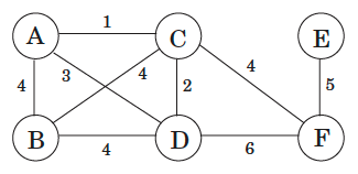
One immediate observation is that the optimal set of edges cannot contain a cycle, because removing an edge from this cycle would reduce the cost without compromising connectivity:
Property 1: Removing a cycle edge cannot disconnect a graph.
So the solution must be connected and acyclic: undirected graphs of this kind are called trees.
Trees (three additional properties)
A tree is an undirected graph that is connected and acyclic. Much of what makes trees so useful is the simplicity of their structure. For instance,
Property 2: A tree on nodes has edges.
This can be seen by building the tree one edge at a time, starting from an empty graph. Initially each of the nodes is disconnected from the others, in a connected component by itself. As edges are added, these components merge. Since each edge unites two different components, exactly edges are added by the time the tree is fully formed.
In a little more detail: When a particular edge comes up, we can be sure that and lie in separate connected components, for otherwise there would already be a path between them and this edge would create a cycle. Adding the edge then merges these two components, thereby reducing the total number of connected components by one. Over the course of this incremental process, the number of components decreases from to one, meaning that edges must have been added along the way.
The converse is also true.
Property 3: Any connected, undirected graph with is a tree.
We just need to show that is acyclic. One way to do this is to run the following iterative procedure on it: while the graph contains a cycle, remove one edge from this cycle. The process terminates with some graph , , which is acyclic and, by Property 1, is also connected. Therefore is a tree, whereupon by Property 2. So , no edges were removed, and was acyclic to start with.
In other words, we can tell whether a connected graph is a tree just by counting how many edges it has. Here's another characterization.
Property 4: An undirected graph is a tree if and only if there is a unique path between any pair of nodes.
In a tree, any two nodes can only have one path between them; for if there were two paths, the union of these paths would contain a cycle.
On the other hand, if a graph has a path between any two nodes, then it is connected. If these paths are unique, then the graph is also acyclic (since a cycle has two paths between any pair of nodes).
The particular tree we want is the one with minimum total weight, known as the minimum spanning tree. Here is its formal definition.
MST Definition
Input: An undirected graph ; edge weights .
Output: A tree , with , that minimizes .
In the preceding example, the minimum spanning tree has a cost of 16:
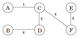
However, this is not the only optimal solution. Can you spot another? (Yes: Delete the edge and replace it with the edge of equivalent value.)
Kruskal's minimum spanning tree algorithm starts with the empty graph and then selects edges from according to the following rule.
Repeatedly add the next lightest edge that doesn't produce a cycle.
In other words, it constructs the tree edge by edge and, apart from taking care to avoid cycles, simply picks whichever edge is cheapest at the moment. This is a greedy algorithm: every decision it makes is the one with the most obvious immediate advantage.
The following figure shows an example:
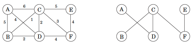
We start with an empty graph and then attempt to add edges in increasing order of weight (ties are broken arbitrarily):
The first two succeed, but the third, , would produce a cycle if added. So we ignore it and move along. The final result is a tree with cost 14, the minimum possible.
The correctness of Kruskal's method follows from a certain cut property [discussed in detail under the template for Prim's algorithm], which is general enough to also justify a whole slew of other minimum spanning tree algorithms.
For Kruskal's algorithm, at any given moment, the edges it has already chosen form a partial solution, a collection of connected components each of which has a tree structure. The next edge to be added connects two of these components; call them and . Since is the lightest edge that doesn't produce a cycle, it is certain to be the lightest edge between and and therefore satisfies the cut property.
Now we fill in some implementation details. At each stage, the algorithm chooses an edge to add to its current partial solution. To do so, it needs to test each candidate edge to see whether the endpoints and lie in different components; otherwise the edge produces a cycle. And once an edge is chosen, the corresponding components need to be merged. What kind of data structure supports such operations?
We will model the algorithm's state as a collection of disjoint sets, each of which contains the nodes of a particular component. Initially each node is in a component by itself:
makeset(x): create a singleton set containing justx.
We repeatedly test pairs of nodes to see if they belong to the same set.
find(x): to which set doesxbelong?
And whenever we add an edge, we are merging two components.
union(x, y): merge the sets containingxandy.
The final algorithm is shown below:
PROCEDURE KRUSKAL (G, w)
Input: A connected undirected graph G = (V, E) with edge weights w_e
Output: A minimum spanning tree defined by the edges X
for all u in V:
makeset(u)
X = {}
sort the edges E by weight
for all edges {u, v} in E, in increasing order of weight:
if find(u) != find(v):
add edge {u, v} to X
union(u, v)
It uses makeset, find, and union operations.
A data structure for disjoint sets (union-find, union by rank)
Note: What follows is an alternative description for how to come up with the union-find data structure in the context of trying to implement Kruskal's algorithm. It may be beneficial to look at the template on this page for the union-find data structure and how to invent it yourself before trying to fully follow the discussion below.
Union by rank:
One way to store a set is as a directed tree (the figure below is a directed-tree representation of two sets and ):
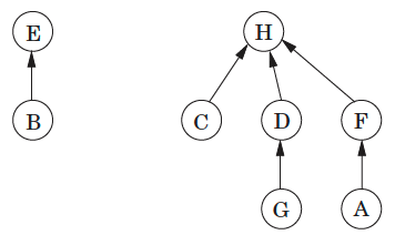
Nodes of the tree are elements of the set, arranged in no particular order, and each has parent pointers that eventually lead up to the root of the tree. This root element is a convenient representative, or name, for the set. It is distinguished from the other elements by the fact that its parent pointer is a self-loop.
In addition to a parent pointer , each node also has a rank that, for the time being, should be interpreted as the height of the subtree hanging from that node.
PROCEDURE MAKESET(x)
pi(x) = x
rank(x) = 0
FUNCTION FIND(x)
while x != pi(x):
x = pi(x)
return x
As can be expected, makeset is a constant-time operation. On the other hand, find follows parent pointers to the root of the tree and therefore takes time proportional to the height of the tree. The tree actually gets built via the third operation, union, and so we must make sure that this procedure keeps trees shallow.
Merging two sets is easy: make the root of one point to the root of the other. But we have a choice here. If the representatives (roots) of the sets are and , do we make point to or the other way around? Since tree height is the main impediment to computational efficiency, a good strategy is to make the root of the shorter tree point to the root of the taller tree. This way, the overall height increases only if the two trees being merged are equally tall. Instead of explicitly computing heights of trees, we will use the rank numbers of their root nodes — which is why this scheme is called union by rank.
PROCEDURE UNION(x,y)
r_x = find(x)
r_y = find(y)
if r_x = r_y: return
if rank(r_x) > rank(r_y):
pi(r_y) = r_x
else:
pi(r_x) = r_y
if rank(r_x) = rank(r_y):
rank(r_y) = rank(r_y) + 1
The figure below illustrates this procedure (a sequence of disjoint-set operations, where superscripts denote rank):
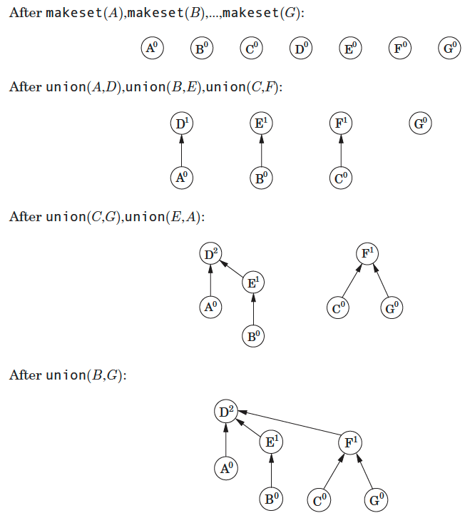
By design, the rank of a node is exactly the height of the subtree rooted at that node. This means, for instance, that as you move up a path toward a root node, the rank values along the way are strictly increasing.
Property 1: For any , .
A root node with rank is created by the merger of two trees with roots of rank . It follows by induction (try it!) that
Property 2: Any root node of rank has at least nodes in its tree.
This extends to internal (nonroot) nodes as well: a node of rank has at least descendants. After all, any internal node was once a root, and neither its rank nor its set of descendants has changed since then. Moreover, different rank- nodes cannot have common descendants, since by Property 1 any element has at most one ancestor of rank . Which means
Property 3: If there are elements overall, there can be at most nodes of rank .
This last observation implies, crucially, that the maximum rank is . Therefore, all the trees have , and this is an upper bound on the running time of find and union.
Path compression:
With the data structure as presented so far, the total time for Kruskal's algorithm becomes for sorting the edges (remember, ) plus another for the union and find operations that dominate the rest of the algorithm. So there seems to be little incentive to make our data structure any more efficient.
But what if the edges are given to us sorted? Or if the weights are small (say, ) so that sorting can be done in linear time? Then the data structure part becomes the bottleneck, and it is useful to think about improving its performance beyond per operation. As it turns out, the improved data structure is useful in many other applications.
But how can we perform union's and find's faster than ? The answer is, by
being a little more careful to maintain our data structure in good shape. As any
housekeeper knows, a little extra effort put into routine maintenance can pay off
handsomely in the long run, by forestalling major calamities. We have in mind a
particular maintenance operation for our union-find data structure, intended to keep
the trees short — during each find, when a series of parent pointers is followed up
to the root of a tree, we will change all these pointers so that they point directly
to the root (the figure shows the effect of path compression, where find(I) is followed by find(K)):
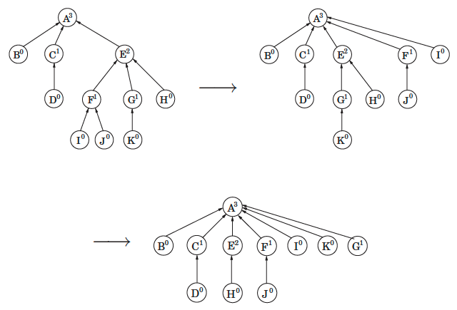
This path compression heuristic only slightly increases the time needed for a find and is easy to code.
FUNCTION FIND(x)
if x != pi(x):
pi(x) = find(pi(x))
return pi(x)
The benefit of this simple alteration is long-term rather than instantaneous and thus necessitates a particular kind of analysis: we need to look at sequences of find and union operations, starting from an empty data structure, and determine the average time per operation. This amortized cost turns out to be just barely more than , down from the earlier .
Think of the data structure as having a "top level" consisting of the root nodes, and below it, the insides of the trees. There is a division of labor: find operations (with or without path compression) only touch the insides of trees, whereas union's only look at the top level. Thus path compression has no effect on union operations and leaves the top level unchanged.
We now know that the ranks of root nodes are unaltered, but what about nonroot nodes? The key point here is that once a node ceases to be a root, it never resurfaces, and its rank is forever fixed. Therefore the ranks of all nodes are unchanged by path compression, even though these numbers can no longer be interpreted as tree heights. In particular, properties 1–3 (concerning trees) still hold.
We can test our template on the graph provided before the pseudocode for Kruskal's algorithm:
def kruskal(graph, num_vertices):
# ...
graph = [
[1, 2, 1], # B - C (1)
[2, 3, 2], # C - D (2)
[1, 3, 2], # B - D (2)
[2, 5, 3], # C - F (3)
[3, 5, 4], # D - F (4)
[4, 5, 4], # E - F (4)
[0, 3, 4], # A - D (4)
[0, 1, 5], # A - B (5)
[2, 4, 5], # C - E (5)
[0, 2, 6], # A - C (6)
]
kruskal(graph, 6) # (14, [(1, 2), (2, 3), (2, 5), (4, 5), (0, 3)])
# [(B, C), (C, D), (C, F), (E, F), (A, D)]
The final edge list returned, namely [(B, C), (C, D), (C, F), (E, F), (A, D)], is the MST, and this confirms the MST shown in the picture.
Time and space complexity
Time: . Dominated by the sorting of edges. Union-Find operations contribute , which is effectively .
Space: .
Note: denotes the inverse Ackermann function.
# T: O(E log E); S: O(V + E)
def kruskal(graph, num_vertices):
uf = UnionFind(num_vertices) # assumes efficient implementation (e.g., union by rank with path compression)
mst = [] # the final MST as a list of edges
mst_cost = 0 # total edge cost of MST
graph.sort(key=lambda edge: edge[2]) # sort edge list before greedily adding edges to MST
for src, dst, wgt in graph: # assumed edge formulation: [source, destination, weight]
if not uf.connected(src, dst): # add minimum edge (src, dst) to MST if src and dst are in separate components
mst.append((src, dst))
mst_cost += wgt
uf.union(src, dst) # connect src and dst so as to be in the same component
return mst_cost, mst
Examples
TBD
Boruvka
Remarks
TBD
# T: O(α(n)) per operation; S: O(n)
class UnionFind:
def __init__(self, num_vertices):
self.root = [i for i in range(num_vertices)]
self.rank = [0] * num_vertices
def find(self, x):
if self.root[x] != x:
self.root[x] = self.find(self.root[x])
return self.root[x]
def union(self, x, y):
root_x = self.find(x)
root_y = self.find(y)
if root_x == root_y:
return False
rank_x = self.rank[root_x]
rank_y = self.rank[root_y]
if rank_x > rank_y:
self.root[root_y] = root_x
elif rank_x < rank_y:
self.root[root_x] = root_y
else:
self.root[root_y] = root_x
self.rank[root_x] += 1
return True
def connected(self, x, y):
return self.find(x) == self.find(y)
def boruvka(edge_list, n):
uf = UnionFind(n) # union-find structure to efficiently manage connected components
mst = [] # list to store edges included in the final returned MST
num_components = n # number of components (starts with n, where each vertex is its own component)
# current edge list to process (size is reduced from phase to phase)
# (used for edge removal optimization)
current_edge_list = [ edge[:] for edge in edge_list ]
# continue until all vertices are connected into a single component
while num_components > 1:
cheapest = [None] * n # initialize cheapest edge for each component to None
# (index corresponds to component's representative or root in union-find structure)
new_edge_list = [] # prepare new edge list for next phase (for edge removal optimization)
# iterate over all edges to find cheapest outgoing edge from each component
for edge in current_edge_list:
u, v, weight = edge
comp_u = uf.find(u) # find component (root) of vertex u
comp_v = uf.find(v) # find component (root) of vertex v
if comp_u != comp_v:# consider edge (u,v) if u and v are in different components
new_edge_list.append(edge) # keep edge for next phase
# check if edge is cheapest for component comp_u
if cheapest[comp_u] is None or is_preferred_over(edge, cheapest[comp_u]):
cheapest[comp_u] = edge
# check if edge is cheapest for component comp_v
if cheapest[comp_v] is None or is_preferred_over(edge, cheapest[comp_v]):
cheapest[comp_v] = edge
# edges connecting vertices within same component are ignored
current_edge_list = new_edge_list # update edge list to only include edges connecting different components
print(cheapest)
print(f'Components before merge: {[uf.find(i) for i in range(n)]}')
# add cheapest edges to MST and merge components
edges_added = False # track whether or not any edges were added in a phase
for i in range(n):
if cheapest[i] is not None:
u, v, weight = cheapest[i]
# attempt to union components
if uf.union(u, v): # (union() returns True if a merge occurs, False otherwise)
mst.append([u, v, weight]) # add edge to MST
num_components -= 1 # decrement component count
edges_added = True # an edge was added to the MST in this pase
print(f'Components after merge: {[uf.find(i) for i in range(n)]}')
# if no edges were added, then MST cannot be formed (graph may be disconnected)
if not edges_added:
return []
return mst
# determines if edge1 is preferred over edge2 (based on weight and tie-breaking rules)
def is_preferred_over(edge1, edge2):
if edge2 is None:
return True
weight1 = edge1[2]
weight2 = edge2[2]
if weight1 < weight2:
return True
elif weight1 > weight2:
return False
else:
return tie_breaking_rule(edge1, edge2)
# tie-breaking rule for when edge weights are equal
# edges are compared based on vertex indices
# (first by smaller vertex index (u), then by larger vertex index (v))
def tie_breaking_rule(edge1, edge2):
u1, v1 = sorted((edge1[0], edge1[1]))
u2, v2 = sorted((edge2[0], edge2[1]))
if u1 < u2:
return True
elif u1 > u2:
return False
else:
return v1 < v2
Examples
TBD
Kosaraju (SCC)
Basic motivation, concepts, and considerations for Kosaraju
The motivation for Kosaraju's algorithm for finding strongly connected components (SCCs), as described below, is largely inspired by this video. My goal here is mostly to provide more explanations and working code. If you watch the video linked above without any context, then it will likely be somewhat hard to follow because it builds off of progress from a few previous videos, namely the following:
- Depth first search (DFS): Covers much of the terminology and notation used below (e.g., edge classifications such as tree edges, back edges, forward edges, and cross edges, as well as discovered and finished times for different vertcies, the
dandfvalues seen in vertices used throughout the example graph in this note, and more) - Kahn's algorithm for topological sorting
- DFS-based algorithm for finding a topological order of a directed acyclic graph
Watching the videos linked above and/or reading the notes for these very topics on this page will go a long way in making the rest of this note make sense.
Kosaraju's algorithm is all about finding strongly connected components, but this does us little good if we do not even know what a component is. In an undirected graph, components are the different connected pieces of the graph. If there's any path from one vertex to another, then these vertices are in the same component:
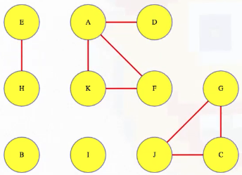
If the entire graph is connected, then it has just one component. One easy way to partition the graph into its separate components is to run depth first search on the entire graph, and each time that a top-level call finds a previously undiscovered vertex, then that vertex's depth first search will discover its entire component.
Below, A discovers D and F directly and then discovers K indirectly, and that is the first component found. Top-level searches for B and C discover their components, but D is already discovered so its top-level search will just exit right away so that we can move on to E (i.e., in the context of executing DFS on an entire graph, we execute top-level searches on each vertex, A through J, in alphabetical order for ease of reference):
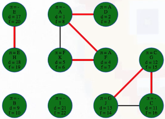
When DFS finishes, we have some tree and back edges (colored red and black above, respectively), and each of the trees in the depth first search forest makes one component:
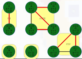
However, if a graph is directed, then how do we actually define what a "component" is?
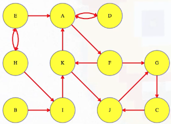
Above, if A has a path to G but G has no path back to A, then are A and G in the same component? We say that two vertices are strongly connected if each has a path to the other (i.e., they lie on some cycle with each other). Vertices in a directed graph are partitioned into strongly connected components — each component is a subset of vertices that can all reach each other. Each vertex will be in exactly one component along with the vertices that it can reach and that can reach it:
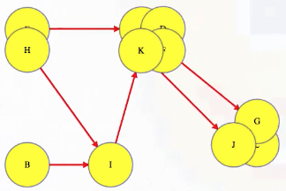
Notice above that A and D are in the same component and so are A and F. Because of this, D and F have to be in the same component. They can each reach each other through their paths to and from A. If a vertex isn't in any cycle, then even if it has edges in and out of it, it's all alone in its own component (e.g., vertex I in our example graph). Our goal is to find strongly connected components from a graph, ideally with an efficient algorithm.
If we don't care about efficiency, then we can come up with an algorithm with relative ease: grab a vertex like A, see what it can reach, maybe with DFS:
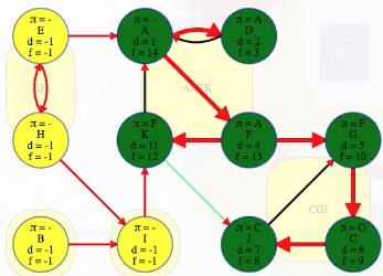
Then, if we reverse the graph (i.e., swap the direction of all edges to create the transpose of the graph) and search the same vertex A again, then we can see what can reach it in the original graph:
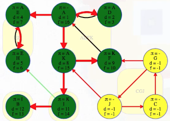
By superimposing one result on to the other, we can see the intersection of those two sets, the vertices that A can reach and that can reach A:
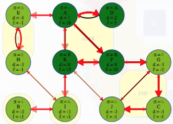
This will conclusively tell us what strongly connected component A belongs to:
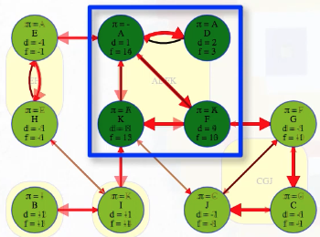
We could do the same search for every vertex in the graph, but we only need to do it once per component. For example, once we know D is in A's component, we don't need to repeat that work on D. To summarize, the following would be an inefficient but doable algorithm:
- Search from a vertex to see what it can reach.
- Search from the same vertex in the reverse graph to see what can reach it.
- Intersect those two sets to find its strongly connected component.
- Repeat with other vertices.
How long this algorithm takes depends on how we implement it, but it would be pretty easy to find one component in time proportional to the size of the graph. Hence, if there are strongly connected components, then we would be looking at time per component, which would give us a total time complexity of .
If we want better efficiency, then let's stop to really think about the strongly connected components. Let's collapse vertices from each component into one "super-vertex" and draw edges between super vertices if there are any edges between their corresponding sets of vertices:
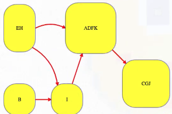
The graph above, the underlying component graph, must be acyclic. Why? Because if it had a cycle, then all vertices from the cycle's corresponding vertices in the original graph could all reach each other through some combination of intra and inter-component edges — all such connected vertices could be collapsed into one component. If the original graph is acyclic, then the underlying component graph looks just like the original graph — every vertex would be its own component.
Both topological order algorithms on this page (i.e., Kahn's algorithm and a DFS-based algorithm) each found topological orders either from the beginning (Kahn) or the end (DFS) of the ordering. Those seemed like easier places to start. Our hope is that it might be easier to find strongly connected components if we do it by topological order for the underlying component graph:
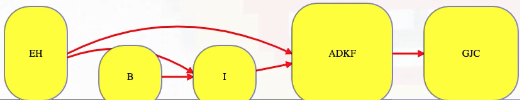
We started this note by finding components in an undirected graph with DFS. In that context, with an undirected graph, we didn't need to intersect the set of vertices from the first search with the vertices from the second search. Let's now consider the following directed graph:
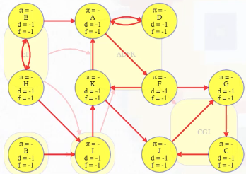
Imagine if we could (magically) start a search on a vertex in the topologically last component, maybe C in the graph above. We would discover C's strongly connected component in time linear to the number of vertices and edges in that component. We wouldn't need to reverse the graph and do another search and find the intersection. We would just discover the component and be done with it because C's component is topologically last, which means the search can't escape it (i.e., its strongly connected component has no outgoing edges, as illustrated in the underlying component graph). So it would be really nice to search it first and mark it as done.
If we topologically order the underlying component graph, then A's component would be second to last, just before C's component. After we've marked C's component, it would be great if we could next search a vertex from A's component — the search would discover all of its component, but it wouldn't rediscover C's component, which was already discovered when we searched C.
Clever Observation (1)
Of course, because we don't know what the components are ahead of time, we don't know how to easily grab a vertex from the topologically last component to search it. Can we figure out some way to topologically sort the underlying component graph even if we don't know the components? For the two common topological ordering algorithms, Kahn's and DFS, each behaves differently if we run it on a graph with cycles. For any vertex on a cycle or even reachable from a cycle, Kahn's algorithm will never get that vertex's in-degree down to 0 so it will never make it into the ordering. We'll end up with an order that only includes the other vertices (i.e., vertices whose in-degree could eventually be made 0).
In the directed graph above, Kahn's algorithm would return just vertex B. That's obviously not too helpful here. On the other hand, the DFS-based topological ordering runs DFS and orders the vertices in the reverse order that they finish. That algorithm will order all the vertices in the graph regardless of cycles; of course, the resultant ordering will not be a topological ordering (because none exists in a graph with cycles), but the ordering is related to the topological ordering of the underlying component graph.
Let's run a DFS on the graph and record the discovery and finish times along with the predecessors and edge classifications (the note on the motivation behind recursive DFS outlines how to do this iteratively) by first representing the graph as an adjacency list of index arrays in code:
graph = [
[3, 5],
[8],
[9],
[0],
[0, 7],
[6, 10],
[2],
[4, 8],
[10],
[6],
[0, 9],
]
lookup = {
-1: ' ',
0: 'A',
1: 'B',
2: 'C',
3: 'D',
4: 'E',
5: 'F',
6: 'G',
7: 'H',
8: 'I',
9: 'J',
10: 'K',
}
Running the aforementioned algorithm yields the following (formatted manually for ease of reference):
"""
( A B C D E F G H I J K
[ 1, 15, 6, 2, 19, 4, 5, 20, 16, 7, 11], # discovered
[14, 18, 9, 3, 22, 13, 10, 21, 17, 8, 12], # finished
[-1, -1, 6, 0, -1, 0, 5, 4, 1, 2, 5], # predecessors
{ # edge classifications
('A', 'D'): 'treeEdge',
('D', 'A'): 'backEdge',
('A', 'F'): 'treeEdge',
('F', 'G'): 'treeEdge',
('G', 'C'): 'treeEdge',
('C', 'J'): 'treeEdge',
('J', 'G'): 'backEdge',
('F', 'K'): 'treeEdge',
('K', 'A'): 'backEdge',
('K', 'J'): 'crossEdge',
('B', 'I'): 'treeEdge',
('I', 'K'): 'crossEdge',
('E', 'A'): 'crossEdge',
('E', 'H'): 'treeEdge',
('H', 'E'): 'backEdge',
('H', 'I'): 'crossEdge'
}
)
"""
This confirms the DFS run on the graph in the video:
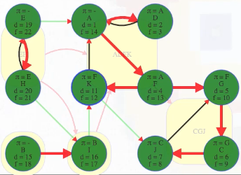
That's where the story would end if we just wanted to run a DFS on the whole graph (i.e., finding discovered and finished times for each vertex as well as their predecessors and edge classifications). But in this case, we also want to consider the discovery and finish times for the underlying component super-vertices. The algorithm itself doesn't have any idea what the components are, but we can just cheat and look at them for now.
Importantly, we can define component discovery and finish times as follows:
- discovered: the first time one of its vertices is discovered
- finished: the last time one of its vertices is finished
Note that within each component those two times come from the same vertex:
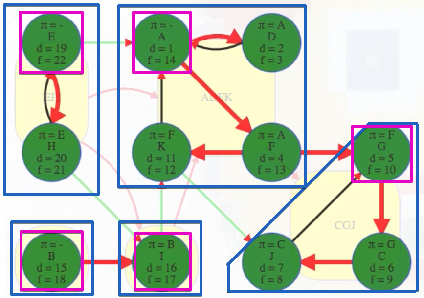
It has to be like that. The first vertex discovered in any component cannot finish being explored until everything it can reach, including all vertices within its component, is finished. Vertices that are discovered later in the component will finish earlier. In the graph above, D is able to finish before other vertices in the same component have been discovered because it only reaches the rest of the component through vertex A. This brings us to the next clever observation.
Clever Observation (2)
For the same reason that DFS topological sort works, DFS will finish underlying components in reverse topological order. Recall the following details about edge classification in terms of the graph we've been analyzing:
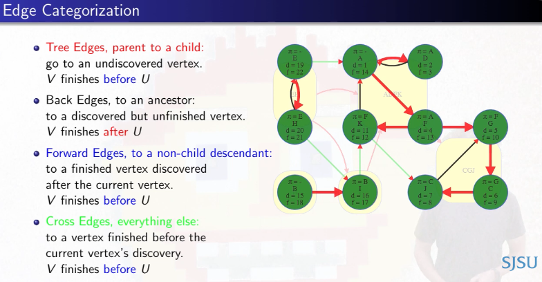
For DFS, tree, forward, and cross edges all have to finish their target vertex before their source vertex. How about back edges? They complete cycles so they all go between two vertices from the same component. Edges between different components have to be something other than a back edge (otherwise the two components could be collapsed into one) — this means that the target vertex and everything it can reach, including that target vertex's entire component, must be finished before the source vertex from the other component is finished. Hence, the source vertex's topologically earlier component has to finish after the target's topologically later component.
Clarification
The previous statement is easiest to understand by means of an example from the graph above. Consider the components represented by super vertices ADFK and CGJ. Now consider the tree edge from F to G or the cross edge from K to J that connect these two different components. As expected, neither of these edges are back edges. The edge (F, G) has F as its source vertex and G as its target vertex; similarly, the edge (K, J) has K as its source vertex and J as its target vertex. As noted above, the target vertex and everything it can reach, including the target vertex's entire component, must be finished before the source vertex from the other component is finished:
(F, G): The source vertexFhas finish time13while the target vertexGand all the vertices in its component have finish times before the source vertex:G,C,Jhave finish times10,9,8, respectively, all indicating they are finished before the source vertexF.(K, J): The source vertexKhas finish time12while the target vertexJand all the vertices in its component have finish times before the source vertex:J,G,Chave finish times8,10,9, respectively, all indicating they are finished before the source vertexK.
Before remarking on the key takeaway, it's a good time to recall that DFS returns a reverse topological ordering. We can't have a topological ordering for the original graph (because it contains cycles), but, as previously mentioned, the underlying component graph is a DAG which means it must have a topological ordering. In the second figure above, if we ordered components left to right by ascending finish times of their first discovered vertex, then we would have CGJ -> ADFK -> I -> B -> EH:
CGJ # G has finish time 10
-> ADFK # A has finish time 14
-> I # I has finish time 17
-> B # B has finish time 18
-> EH # E has finish time 22
But that is the reverse topological ordering. The proper topological ordering is
EH -> B -> I -> ADFK -> CGJ
The key takeaway is the following:
The source vertex's topologically earlier component has to finish after the target's topologically later component.
This should now be clearer in light of the example edges we've been considering:
The source vertex's topologically earlier component [
ADFKin the case of the source verticesFandKfor the edges(F, G)and(K, J)] has to finish after the target's topologically later component [CGJin the case of the target verticesGandJfor the edges(F, G)and(K, J)]
Hence, a component that finishes later actually comes earlier in the final non-reversed topological ordering.
But we still don't know what the components are! Nonetheless, running DFS still tells us something about their topological order anyway (i.e., topological order of the components, not the vertices of the original graph itself). Our goal was to learn enough about the underlying component graph's topological order to grab a vertex from the topologically last component, namely C's component in the example graph we've been considering. But from the finish times we've obtained, it still seems hard to do this effectively. In our graph, for example, vertex D finishes first, but its component is in the middle somewhere. The topologically last component finishes first at time 10 for vertex G, but that's hidden from us because we don't know the components ahead of time, and G isn't the first vertex to finish — vertex D is. Without knowing the components, the finish times don't actually help us in identifying a vertex from the topologically last component, which finishes first.
Clever Observation (3)
However, it's easy for us to promise that E's component finishes last because E itself finishes last. Hence, E's component can go topologically first.
Let's save vertices in the order of their reverse finish times like DFS topological sort does:
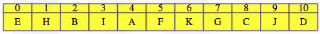
It would be nice to find and delete that entire first component and continue on similar to what we did while developing Kahn's algorithm (see note concerning motivation for Kahn's algorithm). But how do we delete it if we don't know where it starts and ends? Unlike taking a vertex in the topologically last component, if we search a vertex in the topologically first component, then we might search other components too. In the directed graph previously pictured, E would discover everything except B. This brings us to our last clever observation.
Clever Observation (4)
Let , pictured left below, denote the original graph. Now let's reverse to obtain , pictured right below (i.e., we reverse the direction of all edges):
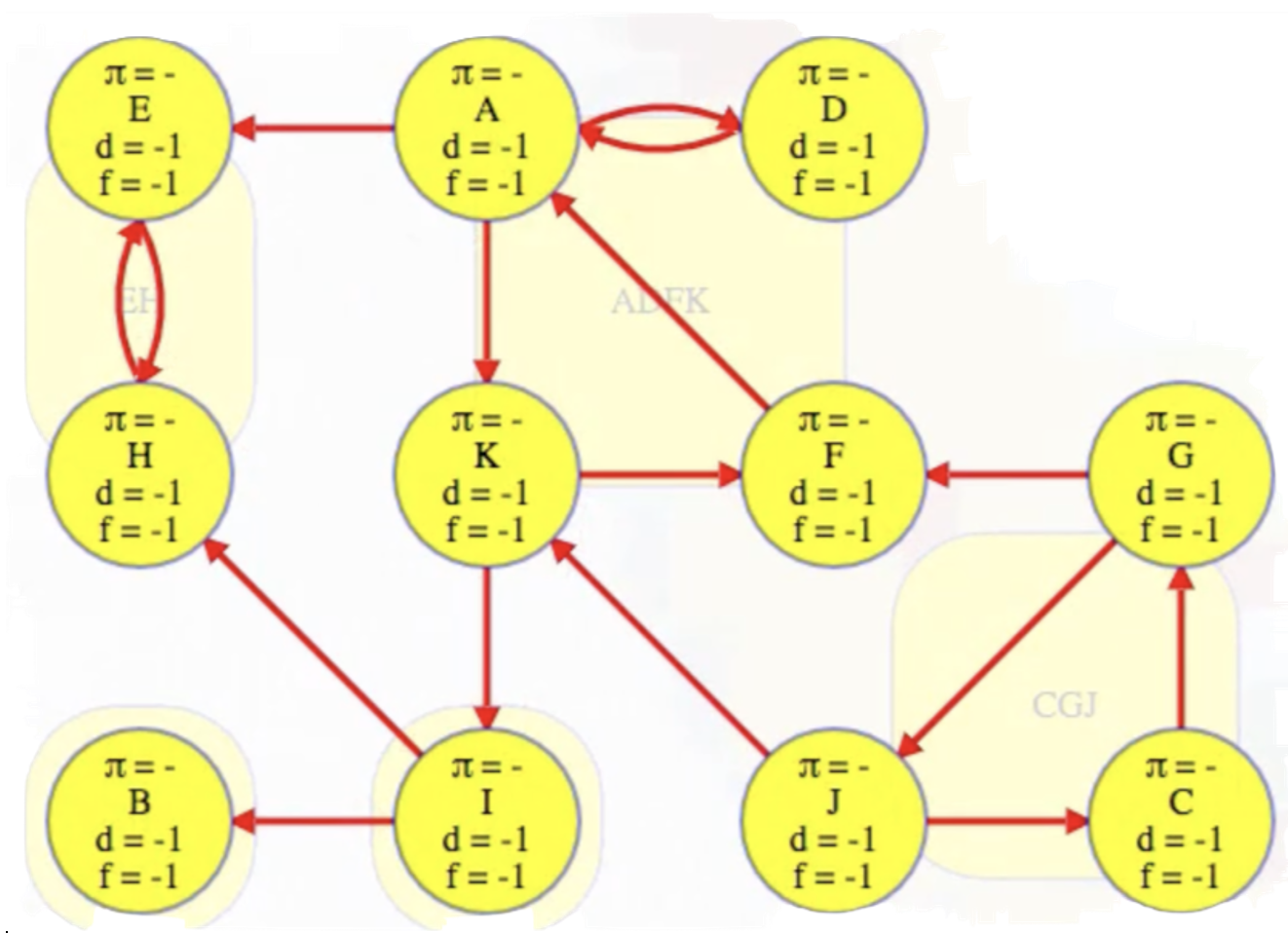
The strongly connected components stay the same. Any two vertices that were on a cycle in are still on a cycle in — the cycle just goes the other way. But the edges in the underlying component graph now go in the opposite direction. The topologically first component that couldn't be reached by any other component (i.e., EH) now can't reach any other component. It is topologically last. So we can grab vertex E, which we know is in the topologically last component in the reversed graph, search it, and bang! We discover its entire strongly connected component:
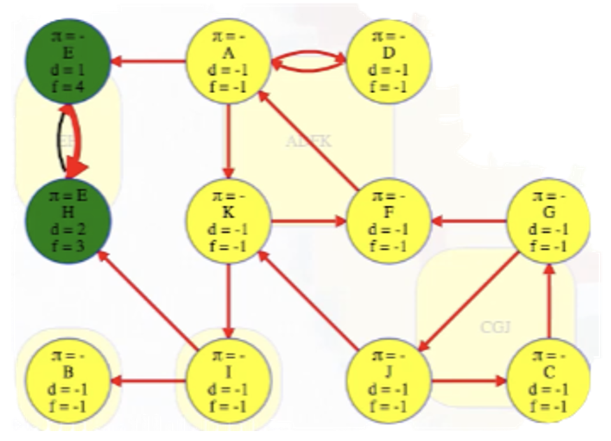
It has no other outgoing edges to other components. Conveniently, the vertex order we saved from our DFS on , the original graph, now lists vertices from the topologically latest components of the reversed graph first. We use that order to search for components in , the reversed graph, and we don't need to delete them from the graph to continue. DFS will mark all vertices in E's component as explored, and then we can just continue top-level searches from the other vertices using the next latest finish time from our saved vertex order.
Continuing our search, we go to H next, but H is already discovered so DFS will ignore it, which is good, because we already know its component! The next vertex we run into that we haven't already discovered is B (i.e., going by the vertex order produced by the first DFS of ). Its component has the second latest finish time so it can be topologically second to last, just before E's component, in the reversed underlying component graph (or second in the original underlying component graph).
Vertex B doesn't have any outgoing edges in the reverse graph, but the next vertex I does. It has edges to both E and B's components, but we already know what those components are. We can't rediscover them. We finish the second DFS on , the reversed graph, taking vertices in the reverse order that they finished the initial DFS on , the original graph. Every time we come across a new top-level vertex that hasn't been previously discovered, it will discover its strongly connected component:
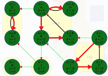
This last part of the algorithm looks just like discovering components in an undirected graph using DFS except we need to do our top-level searches in the specific order given from the earlier DFS. When we finish, the top-level searches that found something, namely E, B, I, A, and G, have no parent nodes (each discovered its own component):
"""
( A B C D E F G H I J K
[ 9, 5, 19, 10, 1, 13, 17, 2, 7, 18, 12], # discovered
[16, 6, 20, 11, 4, 14, 22, 3, 8, 21, 15], # finished
[-1, -1, 9, 0, -1, 10, -1, 4, -1, 6, 0], # predecessors (-1 indicates no parent)
{ # edge classifications
('E', 'H'): 'treeEdge',
('H', 'E'): 'backEdge',
('I', 'B'): 'crossEdge',
('I', 'H'): 'crossEdge',
('A', 'D'): 'treeEdge',
('D', 'A'): 'backEdge',
('A', 'E'): 'crossEdge',
('A', 'K'): 'treeEdge',
('K', 'F'): 'treeEdge',
('F', 'A'): 'backEdge',
('K', 'I'): 'crossEdge',
('G', 'F'): 'crossEdge',
('G', 'J'): 'treeEdge',
('J', 'C'): 'treeEdge',
('C', 'G'): 'backEdge',
('J', 'K'): 'crossEdge
}
)
"""
The DFS forest shows the components with each tree being one component. All edges from one component to another are cross edges:
(A, E) # connects ADFK to EH
(I, H) # connects I to EH
(I, B) # connects I to B
(G, F) # connects CGJ to ADFK
(J, K) # connects CGJ to ADFK
That isn't by chance. The only edge that can go between components in that final search is a cross edge because in the reversed graph each component is explored and finished before any other component has a chance to accidentally discover it by another edge. There can also be cross edges from within a component, but all edges between components will definitely be cross edges. Tree, back, and forward edges all have to go between two vertices in the same component (there simply don't happen to be any forward edges in the sample graph we've been analyzing).
Let's briefly recap the clever observations that have gotten us to this point:
- Clever observation 1: SCCs would be easier to find in reverse topological order for the underlying component graph.
- Clever observation 2: DFS completes the underlying components in reverse topological order.
- Clever observation 3: The component of the last vertex to finish can be topologically first.
- Clever observation 4: has the same underlying SCCs as (in topologically reversed order). The saved DFS order from touches components in a legal reverse topological order.
The clever observations above give us an efficient algorithm for identifying the SCCs of a graph:
- Run DFS on and save the vertex order list by decreasing finish time (finds finish times of unknown components in topological order)
- Find , the reverse graph of ( has the same components but reverses their topological ordering)
- Run DFS on , using the order from step 1 for the top-level calls (finds components in in reverse topological order)
Each successful top-level search discovers a component. Each phase is for total.
In some rough sense, the first DFS on gives us a topological order for the underlying component graph, and that order is the only thing we need from that first search. The second DFS on helps us discover and mark components in topological order. It looks similar to our original inefficient way to just find one strongly connected component, but now we don't have to take any set intersections.
Finally, if we use the template code for Kosaraju's algorithm on the graph we've been discussing, then we get the following:
# E H B I A D K F G J C
[[4, 7], [1], [8], [0, 3, 10, 5], [6, 9, 2]]
# EH -> B -> I -> ADKF -> GJC (topological ordering of component graph)
# T: O(V + E); S: O(V + E)
def kosaraju(graph):
n = len(graph) # graph assumed to be adjacency list of index arrays
visited = [False] * n
finish_order = [] # stack of nodes to be ordered based on finish time (first to last)
# transpose the given graph (reverses all edges)
def transpose_graph(graph):
gt = [[] for _ in range(n)]
for node in range(n):
for nbr in graph[node]:
gt[nbr].append(node) # reverse edge direction
return gt
# first DFS pass: record finish times of nodes
def dfs_first_pass(node):
visited[node] = True # mark current node as visited
for nbr in graph[node]:
if not visited[nbr]:
dfs_first_pass(nbr) # visit all unvisited neighbors
finish_order.append(node) # add node to finish_order after all its descendants are visited
# second DFS pass (on transposed graph): find strongly connected components (SCCs)
def dfs_second_pass(node, component):
visited[node] = True # mark current node as visited
component.append(node) # add node to current SCC
for nbr in graph_transpose[node]:
if not visited[nbr]:
dfs_second_pass(nbr, component) # visit all unvisited neighbors
# step 1: perform DFS on original graph to compute finish times
for node in range(n):
if not visited[node]:
dfs_first_pass(node)
# step 2: create transpose graph (reverse all edges of original graph)
graph_transpose = transpose_graph(graph)
# step 3: process all nodes in order of decreasing finish times
visited = [False] * n # reset visited array for second pass
sccs = [] # initialize collection of SCCs
while finish_order: # process nodes in order of decreasing finish times
node = finish_order.pop() # root (first node) of current SCC
if not visited[node]:
component = [] # store nodes in current SCC
dfs_second_pass(node, component) # perform DFS on transposed graph
sccs.append(component) # add component to overall list of SCCs
return sccs # return complete list of SCCs in topological order
Examples
TBD
Tarjan (SCC)
Standard implementation as it appears on Wikipedia (distinguish between tree edges and back edges)
The following implementation of Tarjan's algorithm more closely aligns with what appears in the algorithm's pseudocode on Wikipedia (the main difference between the implementation below and the core template is that this implementation distinguishes between tree edges and back edges whereas the core template does not; the main difference has been highlighted below):
def tarjan(graph):
n = len(graph) # graph assumed to be adjacency list of index arrays
index = 0 # unique index assigned to each node
indices = [-1] * n # index of each node
low_link = [0] * n # store lowest index reachable from each node
on_stack = [False] * n # boolean array to check if a node is on the stack
stack = [] # stack to keep track of nodes in current SCC
sccs = [] # list to store all SCCs
def dfs(node):
nonlocal index
low_link[node] = index # initialize low_link value of node to be its own index
indices[node] = index # assign smallest unused index to node
index += 1 # increment index value to ensure later nodes have higher index values
stack.append(node) # push node onto the stack
on_stack[node] = True # mark node as being on the stack
# explore all outgoing edges from the node
for neighbor in graph[node]:
if indices[neighbor] == -1: # visit nbr if it has not yet been visited (tree edge)
dfs(neighbor)
low_link[node] = min(low_link[node], low_link[neighbor])
elif on_stack[neighbor]: # nbr is on stack, thus part of current SCC (back edge)
low_link[node] = min(low_link[node], indices[neighbor])
# if node is a root node of an SCC, pop from stack and generate SCC
if indices[node] == low_link[node]:
scc = []
while True:
w = stack.pop()
on_stack[w] = False
scc.append(w)
if w == node:
break
sccs.append(scc) # add SCC to overall list of SCCs
# initialize DFS traversal
for v in range(n):
if indices[v] == -1:
dfs(v)
return sccs # return list of SCCs
Slight divergence from core template below to William Fiset's template (return SCCs not low-link values)
The core template for Tarjan's SCC algorithm is based on the algorithm presented in William Fiset's video, where there's not an explicit distinction between tree edges and back edges when low-link values are updated. However, the core template differs slightly in that what is ultimately returned is not a list of the node's low-link values (where equivalent low-link values means those nodes are in the same SCC); instead, the collection of SCCs itself is returned. To recover the original template from the video, all we have to do is delete three lines from the core template (highlighted in red below) and modify one line (the last line, highlighted in yellow, where we return the list of low-link values instead of the list of SCCs):
def tarjan_old(graph):
n = len(graph) # graph assumed to be adjacency list of index arrays
index = 0 # unique index assigned to each node
indices = [-1] * n # index of each node
low_link = [0] * n # store lowest index reachable from each node
on_stack = [False] * n # boolean array to check if a node is on the stack
stack = [] # stack to keep track of nodes in current SCC
sccs = [] # list to store all SCCs
def dfs(node):
nonlocal index
low_link[node] = index # initialize low_link value of node to be its own index
indices[node] = index # assign smallest unused index to node
index += 1 # increment index value to ensure later nodes have higher index values
stack.append(node) # push node onto the stack
on_stack[node] = True # mark node as being on the stack
# explore all outgoing edges from the node
for nbr in graph[node]:
if indices[nbr] == -1: # visit nbr if it has not yet been visited
dfs(nbr)
if on_stack[nbr]: # nbr is on stack, thus part of current SCC (minimize low-link on callback)
low_link[node] = min(low_link[node], low_link[nbr])
# if node is a root node of an SCC, pop from stack and generate SCC
if indices[node] == low_link[node]:
scc = []
while stack:
scc_nbr = stack.pop()
on_stack[scc_nbr] = False
low_link[scc_nbr] = indices[node]
scc.append(scc_nbr)
if scc_nbr == node:
break
sccs.append(scc) # add SCC to overall list of SCCs
# initialize DFS traversal
for v in range(n):
if indices[v] == -1:
dfs(v)
return low_link
# T: O(V + E); S: O(V)
def tarjan(graph):
n = len(graph) # graph assumed to be adjacency list of index arrays
node_id = 0 # unique node_id assigned to each node
ids = [-1] * n # id of each node
low_link = [0] * n # store lowest id node reachable from each node
on_stack = [False] * n # boolean array to check if a node is on the stack
stack = [] # stack to keep track of nodes in current SCC
sccs = [] # list to store all SCCs
def dfs(node):
nonlocal node_id
low_link[node] = node_id # initialize low_link value of node to be its own node_id
ids[node] = node_id # assign smallest unused node_id to node
node_id += 1 # increment node_id value to ensure later nodes have higher node_id values
stack.append(node) # push node onto the stack
on_stack[node] = True # mark node as being on the stack
# explore all outgoing edges from the node
for nbr in graph[node]:
if ids[nbr] == -1: # visit nbr if it has not yet been visited
dfs(nbr)
if on_stack[nbr]: # nbr is on stack, thus part of current SCC (minimize low-link on callback)
low_link[node] = min(low_link[node], low_link[nbr])
# if node is a root node of an SCC, pop from stack and generate SCC
if ids[node] == low_link[node]:
scc = []
while stack:
scc_nbr = stack.pop()
on_stack[scc_nbr] = False
low_link[scc_nbr] = ids[node]
scc.append(scc_nbr)
if scc_nbr == node:
break
sccs.append(scc) # add SCC to overall list of SCCs
# initialize top-level DFS traversals
for v in range(n):
if ids[v] == -1:
dfs(v)
return sccs # return list of SCCs
Examples
TBD
Implicit
Remarks
TBD
TBD
Examples
LC 752. Open the Lock (✓)
You have a lock in front of you with 4 circular wheels. Each wheel has 10 slots: '0', '1', '2', '3', '4', '5', '6', '7', '8', '9'. The wheels can rotate freely and wrap around: for example we can turn '9' to be '0', or '0' to be '9'. Each move consists of turning one wheel one slot.
The lock initially starts at '0000', a string representing the state of the 4 wheels.
You are given a list of deadends dead ends, meaning if the lock displays any of these codes, the wheels of the lock will stop turning and you will be unable to open it.
Given a target representing the value of the wheels that will unlock the lock, return the minimum total number of turns required to open the lock, or -1 if it is impossible.
class Solution:
def openLock(self, deadends: List[str], target: str) -> int:
def neighbors(node):
ans = []
for i in range(4):
num = int(node[i])
for change in [-1, 1]:
x = (num + change) % 10
ans.append(node[:i] + str(x) + node[i + 1:])
return ans
if "0000" in deadends:
return -1
queue = deque([("0000", 0)])
seen = set(deadends)
seen.add("0000")
while queue:
node, steps = queue.popleft()
if node == target:
return steps
for neighbor in neighbors(node):
if neighbor not in seen:
seen.add(neighbor)
queue.append((neighbor, steps + 1))
return -1
The solution above is quite Pythonic. The key insight in this problem is to view each combination as a node or state we want to visit once. A node's neighbors will be all nodes one letter change away. The trickier part of the problem becomes making the string manipulations effectively and actually generating the neighbors. The neighbors function above does this effectively even though (num + change) % 10 seems odd at first because of how Python's modulus operator % operates — its definition is floored, which means, for example, that -1 % 10 == 9. In general, floored division means the remainder procured by the modulus operator will always have the same sign as the divisor. We could change (num + change) % 10 to (num + change + 10) % 10 to explicitly avoid this confusion if we wanted to.
Another approach is much less clean but also still effective in achieving the desired end result:
class Solution:
def openLock(self, deadends: List[str], target: str) -> int:
def dial_up_down(str_num):
num = int(str_num)
if 1 <= num <= 8:
return str(num - 1), str(num + 1)
else:
if num == 0:
return '9', '1'
else:
return '8', '0'
seen = {'0000'}
deadends = set(deadends)
queue = deque([('0000', 0)])
if target in deadends or '0000' in deadends:
return -1
while queue:
combination, moves = queue.popleft()
if combination == target:
return moves
candidates = []
combination = list(combination)
for i in range(len(combination)):
char = combination[i]
up, down = dial_up_down(char)
new_candidate_up = combination[:]
new_candidate_up[i] = up
new_candidate_down = combination[:]
new_candidate_down[i] = down
candidates.append("".join(new_candidate_up))
candidates.append("".join(new_candidate_down))
for candidate in candidates:
if candidate not in seen and candidate not in deadends:
seen.add(candidate)
queue.append((candidate, moves + 1))
return -1
LC 399. Evaluate Division (✓)
You are given an array of variable pairs equations and an array of real numbers values, where equations[i] = [Ai, Bi] and values[i] represent the equation Ai / Bi = values[i]. Each Ai or Bi is a string that represents a single variable.
You are also given some queries, where queries[j] = [Cj, Dj] represents the jth query where you must find the answer for Cj / Dj = ?.
Return the answers to all queries. If a single answer cannot be determined, return -1.0.
Note: The input is always valid. You may assume that evaluating the queries will not result in division by zero and that there is no contradiction.
class Solution:
def calcEquation(self, equations: List[List[str]], values: List[float], queries: List[List[str]]) -> List[float]:
def build_graph(edges, weights):
graph = defaultdict(dict)
for i in range(len(edges)):
num, denom = edges[i]
weight = weights[i]
graph[num][denom] = weight
graph[denom][num] = 1 / weight
return graph
def answer_query(query):
num, denom = query
if num not in graph or denom not in graph:
return -1
seen = {num}
queue = deque([(num, 1)])
while queue:
node, result = queue.popleft()
if node == denom:
return result
for neighbor in graph[node]:
if neighbor not in seen:
seen.add(neighbor)
queue.append((neighbor, result * graph[node][neighbor]))
return -1
graph = build_graph(equations, values)
return [ answer_query(query) for query in queries ]
This is kind of a wild problem. It takes a lot of imagination to view it as a graph problem at first. The idea is that each element of a quotient (i.e., numerator and denominator) is a node. An edge is the ratio of numerator to denominator as well as denominator to numerator (we view the equations provided as an edge list of undirected edges). Each edge is weighted — the quotient value is the weight.
For example, if we're given that and , then we can model the process of trying to solve for as a graph traversal problem:
The idea is to start at node a, the numerator, and try to eventually reach node c, the denominator, by traveling along the weighted edges. As the diagram above shows, we should have , which we get by starting from a with a product of and then multiplying it by the edge weights as we go: .
The BFS solution above is rather clean, but the DFS solution is arguably more intuitive in a sense (even though it may be slightly harder to code) because we're basically trying to determine whether or not there exists a path from the numerator to the denominator:
class Solution:
def calcEquation(self, equations: List[List[str]], values: List[float], queries: List[List[str]]) -> List[float]:
def build_graph(edges, weights):
graph = defaultdict(dict)
for i in range(len(edges)):
num, denom = edges[i]
weight = weights[i]
graph[num][denom] = weight
graph[denom][num] = 1 / weight
return graph
def answer_query(query):
num, denom = query
if num not in graph or denom not in graph:
return -1
seen = {num}
def dfs(node):
if node == denom:
return 1
for neighbor in graph[node]:
if neighbor not in seen:
seen.add(neighbor)
result = dfs(neighbor)
if result != -1:
return result * graph[node][neighbor]
return -1
return dfs(num)
graph = build_graph(equations, values)
return [ answer_query(query) for query in queries ]
LC 433. Minimum Genetic Mutation (✓)
A gene string can be represented by an 8-character long string, with choices from "A", "C", "G", "T".
Suppose we need to investigate about a mutation (mutation from "start" to "end"), where ONE mutation is defined as ONE single character changed in the gene string.
For example, "AACCGGTT" -> "AACCGGTA" is 1 mutation.
Also, there is a given gene "bank", which records all the valid gene mutations. A gene must be in the bank to make it a valid gene string.
Now, given 3 things - start, end, bank, your task is to determine what is the minimum number of mutations needed to mutate from "start" to "end". If there is no such a mutation, return -1.
Note:
- Starting point is assumed to be valid, so it might not be included in the bank.
- If multiple mutations are needed, all mutations during in the sequence must be valid.
- You may assume start and end string is not the same.
class Solution:
def minMutation(self, startGene: str, endGene: str, bank: List[str]) -> int:
seen = {startGene}
bank = set(bank)
queue = deque([(startGene, 0)])
while queue:
node, mutations = queue.popleft()
if node == endGene:
return mutations
for char in 'ACGT':
for i in range(8):
neighbor = node[:i] + char + node[i+1:]
if neighbor not in seen and neighbor in bank:
seen.add(neighbor)
queue.append((neighbor, mutations + 1))
return -1
It's easy to over-complicate this problem. The core idea is that each gene is a node and nodes are connected by single-difference mutations. The solution above uses the if neighbor not in seen to its advantage to effectively bypass logic for avoiding the consideration of the same gene more than once. That is, for char in 'ACGT' means char will obviously take on values 'A', 'C', 'G', and 'T' even though the character for the current gene in this place is one of these characters. But since the the current node has already been seen, we will not continue a search from it. It's a clever way to simplify the rest of the logic. The 8 in for i in range(8) is due to the fact that each gene string is 8 characters long.
Here's a longer and more complicated (not recommended) solution:
class Solution:
def minMutation(self, startGene: str, endGene: str, bank: List[str]) -> int:
def get_neighbors(node):
neighbors = []
for i in range(8):
for j in range(3):
char_mutation = code_to_char[(char_to_code[node[i]] + (j + 1)) % 4]
gene_mutation = node[:i] + char_mutation + node[i+1:]
if gene_mutation in bank:
neighbors.append(gene_mutation)
return neighbors
char_to_code = { 'A': 0, 'C': 1, 'G': 2, 'T': 3 }
code_to_char = { 0: 'A', 1: 'C', 2: 'G', 3: 'T' }
bank = set(bank)
seen = {startGene}
queue = deque([(startGene, 0)])
while queue:
node, mutations = queue.popleft()
if node == endGene:
return mutations
for neighbor in get_neighbors(node):
if neighbor not in seen:
seen.add(neighbor)
queue.append((neighbor, mutations + 1))
return -1
LC 1306. Jump Game III (✓)
Given an array of non-negative integers arr, you are initially positioned at start index of the array. When you are at index i, you can jump to i + arr[i] or i - arr[i], check if you can reach to any index with value 0.
Notice that you can not jump outside of the array at any time.
class Solution:
def canReach(self, arr: List[int], start: int) -> bool:
def valid(idx):
return 0 <= idx < n
n = len(arr)
seen = {start}
queue = deque([start])
while queue:
idx = queue.popleft()
if arr[idx] == 0:
return True
for neighbor in [ idx - arr[idx], idx + arr[idx] ]:
if valid(neighbor) and neighbor not in seen:
seen.add(neighbor)
queue.append(neighbor)
return False
The BFS solution above is a natural solution for this disguised graph problem.
LC 2101. Detonate the Maximum Bombs (✓)
You are given a list of bombs. The range of a bomb is defined as the area where its effect can be felt. This area is in the shape of a circle with the center as the location of the bomb.
The bombs are represented by a 0-indexed 2D integer array bombs where bombs[i] = [xi, yi, ri]. xi and yi denote the X-coordinate and Y-coordinate of the location of the ith bomb, whereas ri denotes the radius of its range.
You may choose to detonate a single bomb. When a bomb is detonated, it will detonate all bombs that lie in its range. These bombs will further detonate the bombs that lie in their ranges.
Given the list of bombs, return the maximum number of bombs that can be detonated if you are allowed to detonate only one bomb.
class Solution:
def maximumDetonation(self, bombs: List[List[int]]) -> int:
def build_adj_list(edges):
graph = defaultdict(list)
n = len(edges)
for i in range(n):
x1, y1, r1 = bombs[i]
for j in range(i + 1, n):
x2, y2, r2 = bombs[j]
dist = ((x2-x1) ** 2 + (y2-y1) ** 2) ** (1/2)
if r1 >= dist:
graph[i].append(j)
if r2 >= dist:
graph[j].append(i)
return graph
def bombs_detonated(bomb):
seen = {bomb}
queue = deque([(bomb)])
count = 0
while queue:
node = queue.popleft()
count += 1
for neighbor in graph[node]:
if neighbor not in seen:
seen.add(neighbor)
queue.append(neighbor)
return count
graph = build_adj_list(bombs)
return max(bombs_detonated(bomb) for bomb in range(len(bombs)))
Time to remember what the distance between two points is! But for real. The idea here is that each bomb is a node and bomb A is connected to bomb B if bomb B lies within bomb A's blast radius (and vice-verse, indicating we should use a directed graph to model this problem). We then explore what happens when any single bomb is detonated — how many bombs in total will be detonated after any one bomb is detonated? We want the maximum.
We can use a BFS or DFS to answer this question here. The approach above uses a BFS. One small edge case to be aware of is that nothing prevents two bombs from being placed at the exact same location and with the same radius; that is, the entries in bombs will be identical, but they will need to be treated separately. Hence, when we build our graph, we should use each bomb's index as its node label as opposed to a tuple for the bomb. Just because a tuple is immutable/hashable does not mean we should use it in such a way; additionally, if we use tuples for each bomb, then we fail to take into account when two bombs can be in the same location and with the same radius.
General
Remarks
TBD
Examples
LC 1557. Minimum Number of Vertices to Reach All Nodes (✓)
Given a directed acyclic graph, with n vertices numbered from 0 to n-1, and an array edges where edges[i] = [fromi, toi] represents a directed edge from node fromi to node toi.
Find the smallest set of vertices from which all nodes in the graph are reachable. It's guaranteed that a unique solution exists.
Notice that you can return the vertices in any order.
class Solution:
def findSmallestSetOfVertices(self, n: int, edges: List[List[int]]) -> List[int]:
indegrees = [0] * n
for _, destination in edges:
indegrees[destination] += 1
return [ node for node in range(n) if indegrees[node] == 0 ]
Arguably the hardest part of this problem is actually understanding what it's really asking for:
Find the smallest set of vertices from which all nodes in the graph are reachable. It's guaranteed that a unique solution exists. Notice that you can return the vertices in any order.
What does this really mean? It essentially means that all nodes that have no inbound neighboring nodes will comprise the smallest set of vertices we seek. How? Because these nodes only have outbound connections to all other nodes (they are not reachable from any other nodes). Hence, the problem boils down to finding all nodes that have an indegree of 0, as demonstrated above.
LC 997. Find the Town Judge (✓) ★★
In a town, there are N people labelled from 1 to N. There is a rumor that one of these people is secretly the town judge.
If the town judge exists, then:
- The town judge trusts nobody.
- Everybody (except for the town judge) trusts the town judge.
- There is exactly one person that satisfies properties 1 and 2.
You are given trust, an array of pairs trust[i] = [a, b] representing that the person labelled a trusts the person labelled b.
If the town judge exists and can be identified, return the label of the town judge. Otherwise, return -1.
class Solution:
def findJudge(self, n: int, trust: List[List[int]]) -> int:
if len(trust) < n - 1:
return -1
def sum_in_out_degrees(edges):
degree_sum = defaultdict(int)
for truster, trusted in edges:
degree_sum[truster] -= 1 # subtract 1 for outdegree
degree_sum[trusted] += 1 # add 1 for indegree
return degree_sum
lookup = sum_in_out_degrees(trust)
for person in range(1, n + 1):
if lookup[person] == n - 1:
return person
return -1
This is a great problem where you can really get creative in how you solve it. The key insight is to recognize that the town judge, if that person exists, must have an indegree of n - 1 and an outdegree of 0. We can go about computing that in a few different ways, but the approach above is slick in that it tracks the degree total for each person, where 1 is added if the person is being trusted or subtracts 1 if the person is doing the trusting.
The result is that the town judge will have a degree total of n - 1 (i.e., this person is being trusted n - 1 times while having never trusted anyone), but this cannot be possible for anyone else. A longer, slightly less efficient approach (albeit in the same complexity classes in terms of time and space) is to separately maintain the indegree and outdegree counts:
class Solution:
def findJudge(self, n: int, trust: List[List[int]]) -> int:
if len(trust) < n - 1:
return -1
def degree_lookup(edges):
lookup = defaultdict(lambda: [0,0]) # [indegree, outdegree]
for truster, trusted in edges:
lookup[truster][1] += 1
lookup[trusted][0] += 1
return lookup
lookup = degree_lookup(trust)
for person in range(1, n + 1):
if lookup[person][0] == n - 1 and lookup[person][1] == 0:
return person
return -1
LC 1615. Maximal Network Rank (✓)
There is an infrastructure of n cities with some number of roads connecting these cities. Each roads[i] = [ai, bi] indicates that there is a bidirectional road between cities ai and bi.
The network rank of two different cities is defined as the total number of directly connected roads to either city. If a road is directly connected to both cities, it is only counted once.
The maximal network rank of the infrastructure is the maximum network rank of all pairs of different cities.
Given the integer n and the array roads, return the maximal network rank of the entire infrastructure.
class Solution:
def maximalNetworkRank(self, n: int, roads: List[List[int]]) -> int:
def build_adj_list(edges):
graph = defaultdict(set)
for node, neighbor in edges:
graph[node].add(neighbor)
graph[neighbor].add(node)
return graph
graph = build_adj_list(roads)
max_rank = 0
for city in range(n):
city_rank = len(graph[city])
for next_city in range(city + 1, n):
next_city_rank = len(graph[next_city])
rank = city_rank + next_city_rank
if city in graph[next_city]:
rank -= 1
max_rank = max(max_rank, rank)
return max_rank
It's easy to get tripped up in this problem and immediately spring for a DFS, where we then count the total number of outdegrees for neighboring nodes (minus 1 to not overcount the shared outdegree to each other), but the fatal flaw here is highlighted in the problem's third example on LeetCode:
All the cities do not have to be connected.
This means the approach remarked on above will work for cities that are connected, but it will not work for cities that are not connected. If cities are not connected, then we'll want the sum of the outdegrees for two cities and we won't have to subtract 1 because no edge will be shared between them. Point being: there's not a nice way of dealing with this problem other than iterating through all pairs of points to see what the maximal combination is. The rank of each pair is the sum of their outdegrees and then we subtract 1 if they happen to be neighbors (this is why the adjacency representation of the graph uses sets for neighbors instead of lists).
LC 463. Island Perimeter (✓) ★★
You are given row x col grid representing a map where grid[i][j] = 1 represents land and grid[i][j] = 0 represents water.
Grid cells are connected horizontally/vertically (not diagonally). The grid is completely surrounded by water, and there is exactly one island (i.e., one or more connected land cells).
The island doesn't have "lakes", meaning the water inside isn't connected to the water around the island. One cell is a square with side length 1. The grid is rectangular, width and height don't exceed 100. Determine the perimeter of the island.
class Solution:
def islandPerimeter(self, grid: List[List[int]]) -> int:
WATER = 0
LAND = 1
rows = len(grid)
cols = len(grid[0])
island_perimeter = 0
ISLAND_FOUND = False
for row in range(rows):
ROW_ISLAND = False
for col in range(cols):
if grid[row][col] == LAND:
contribution = 4
ISLAND_FOUND = True
ROW_ISLAND = True
if row > 0 and grid[row - 1][col] == LAND:
contribution -= 2
if col > 0 and grid[row][col - 1] == LAND:
contribution -= 2
island_perimeter += contribution
if ISLAND_FOUND and not ROW_ISLAND:
return island_perimeter
return island_perimeter
The editorial solution (approach 2) explains the procedure above effectively. The idea is to purposely count each square as contributing 4 to the total parameter but to subtract away 2 when required (we only have to look at squares up and to the left since we're processing the grid top to bottom and from left to right):
Slide 1
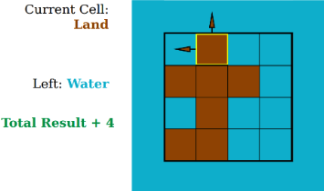
This approach is really quite clever and hard to imagine coming up with in an interview (the WATER variable above is not necessary and is included mostly for the sake of clarity). A more likely solution would be the following where each square's perimeter contribution is directly calculated (we start with a contribution of 4 for each square, as above, but we subtract away 1 whenever adjacent land is encountered):
class Solution:
def islandPerimeter(self, grid: List[List[int]]) -> int:
WATER = 0
LAND = 1
rows = len(grid)
cols = len(grid[0])
island_perimeter = 0
ISLAND_FOUND = False
for row in range(rows):
ROW_ISLAND = False
for col in range(cols):
if grid[row][col] == LAND:
contribution = 4
ISLAND_FOUND = True
ROW_ISLAND = True
up = WATER if row == 0 else grid[row - 1][col]
down = WATER if row == rows - 1 else grid[row + 1][col]
left = WATER if col == 0 else grid[row][col - 1]
right = WATER if col == cols - 1 else grid[row][col + 1]
island_perimeter += (contribution - (up + down + left + right))
if ISLAND_FOUND and not ROW_ISLAND:
return island_perimeter
return island_perimeter
The real trap for this problem is to immediately pursue an overly complicated DFS solution:
class Solution:
def islandPerimeter(self, grid: List[List[int]]) -> int:
def in_bounds(row, col):
return 0 <= row < m and 0 <= col < n
def is_water(row, col):
return not in_bounds(row, col) or grid[row][col] == 0
def is_land(row, col):
return in_bounds(row, col) and grid[row][col] == 1
def find_island(mat):
for i in range(m):
for j in range(n):
if mat[i][j] == 1:
return i, j
def perimeter_contribution(row, col):
above = row - 1, col
below = row + 1, col
left = row, col - 1
right = row, col + 1
perimeter = 0
if is_water(*above):
perimeter += 1
if is_water(*below):
perimeter += 1
if is_water(*left):
perimeter += 1
if is_water(*right):
perimeter += 1
return perimeter
def dfs(row, col):
for dr, dc in dirs:
next_row, next_col = row + dr, col + dc
if (next_row, next_col) not in seen and is_land(next_row, next_col):
nonlocal total_perimeter
total_perimeter += perimeter_contribution(next_row, next_col)
seen.add((next_row, next_col))
dfs(next_row, next_col)
dirs = [(-1,0),(1,0),(0,-1),(0,1)]
m = len(grid)
n = len(grid[0])
island_entry = find_island(grid)
seen = {(island_entry)}
total_perimeter = perimeter_contribution(*island_entry)
dfs(*island_entry)
return total_perimeter
The solution above would be more relevant if we were tasked with, say, finding the maximum perimeter of a number of different islands (i.e., connected components).
Greedy algorithms
Remarks
TBD
# TBD
Examples
LC 2126. Destroying Asteroids (✓)
You are given an integer mass, which represents the original mass of a planet. You are further given an integer array asteroids, where asteroids[i] is the mass of the ith asteroid.
You can arrange for the planet to collide with the asteroids in any arbitrary order. If the mass of the planet is greater than or equal to the mass of the asteroid, the asteroid is destroyed and the planet gains the mass of the asteroid. Otherwise, the planet is destroyed.
Return true if all asteroids can be destroyed. Otherwise, return false.
class Solution:
def asteroidsDestroyed(self, mass: int, asteroids: List[int]) -> bool:
asteroids.sort()
for asteroid in asteroids:
if asteroid > mass:
return False
mass += asteroid
return True
If our planet is not at least as heavy as the smallest asteroid, then it's clearly impossible to destroy all asteroids. The strategy is to destroy and consume the smallest asteroids first, thus ensuring we can destroy as many asteroids as possible. The solution to this problem naturally lends itself to a greedy approach.
LC 2294. Partition Array Such That Maximum Difference Is K (✓)
You are given an integer array nums and an integer k. You may partition nums into one or more subsequences such that each element in nums appears in exactly one of the subsequences.
Return the minimum number of subsequences needed such that the difference between the maximum and minimum values in each subsequence is at most k.
A subsequence is a sequence that can be derived from another sequence by deleting some or no elements without changing the order of the remaining elements.
class Solution:
def partitionArray(self, nums: List[int], k: int) -> int:
nums.sort()
ans = 1
curr_min = nums[0]
for i in range(1, len(nums)):
if nums[i] - curr_min > k:
ans += 1
curr_min = nums[i]
return ans
Intuitively, it makes sense that we would like to cover as many numbers as possible for each subsequence that we could create. We could sort the input and then bunch as many items together as possible whose min-max difference is at most k. The solution above does just that.
LC 502. IPO (✓) ★
Suppose LeetCode will start its IPO soon. In order to sell a good price of its shares to Venture Capital, LeetCode would like to work on some projects to increase its capital before the IPO. Since it has limited resources, it can only finish at most k distinct projects before the IPO. Help LeetCode design the best way to maximize its total capital after finishing at most k distinct projects.
You are given several projects. For each project i, it has a pure profit Pi and a minimum capital of Ci is needed to start the corresponding project. Initially, you have W capital. When you finish a project, you will obtain its pure profit and the profit will be added to your total capital.
To sum up, pick a list of at most k distinct projects from given projects to maximize your final capital, and output your final maximized capital.
class Solution:
def findMaximizedCapital(self, k: int, w: int, profits: List[int], capital: List[int]) -> int:
n = len(profits)
projects = []
for i in range(n):
projects.append((capital[i], profits[i]))
projects.sort()
max_heap = []
i = 0
for _ in range(k):
# push projects to the max heap (based on profit) that we have the capital to start
while i < n and w >= projects[i][0]:
heapq.heappush(max_heap, -projects[i][1])
i += 1
# not enough capital to complete anymore projects
if not max_heap:
return w
w -= heapq.heappop(max_heap)
return w
This problem is rather confusing at first because the capital used to start a project is not deducted from the running capital total; hence, all we really need to do is maximize the profit we can obtain at each step. Sort the capital input array in ascending order and use a max heap to keep track of projects and the profits that can be obtained. The strategy is basically to keep pushing profit-based items (i.e., projects) to the max heap so long as we have the capital to start such projects. As soon as we don't have enough capital to cover the next project, we simply pop the item from the heap that gives us the maximal profit that we can cover — as noted above, we also do not deduct the capital just used to obtain profit. This means we're always starting projects for which we can gain the most profit.
LC 1481. Least Number of Unique Integers after K Removals (✓)
Given an array of integers arr and an integer k. Find the least number of unique integers after removing exactly k elements.
class Solution:
def findLeastNumOfUniqueInts(self, arr: List[int], k: int) -> int:
freqs = defaultdict(int)
for num in arr:
freqs[num] += 1
freqs = sorted(freqs.values(), reverse=True)
while k > 0:
freq = freqs[-1]
k -= freq
if k < 0:
return len(freqs)
freqs.pop()
return len(freqs)
The core idea in this problem is to first count the frequency with which each number occurs and then to remove numbers one at a time from least frequent to most frequent. A variety of ways exist for doing this (e.g., reverse sorting as above and then popping, using a min heap, etc.). But the main greedy strategy is to remove the least frequently occurring numbers first.
LC 881. Boats to Save People (✓)
You are given an array people where people[i] is the weight of the ith person, and an infinite number of boats where each boat can carry a maximum weight of limit. Each boat carries at most two people at the same time, provided the sum of the weight of those people is at most limit.
Return the minimum number of boats to carry every given person.
class Solution:
def numRescueBoats(self, people: List[int], limit: int) -> int:
boats = 0
people.sort()
lightest = 0
heaviest = len(people) - 1
while lightest <= heaviest:
if people[heaviest] + people[lightest] <= limit:
lightest += 1
heaviest -= 1
boats += 1
return boats
The solution editorial highlights the key ideas best:
If the heaviest person can share a boat with the lightest person, then do so. Otherwise, the heaviest person can't pair with anyone, so they get their own boat.
The reason this works is because if the lightest person can pair with anyone, they might as well pair with the heaviest person.
LC 1323. Maximum 69 Number (✓)
Given a positive integer num consisting only of digits 6 and 9.
Return the maximum number you can get by changing at most one digit (6 becomes 9, and 9 becomes 6).
class Solution:
def maximum69Number(self, num: int) -> int:
pos = 0
first_six_pos = -1
ref_num = num
while num > 0:
if num % 10 == 6:
first_six_pos = pos
num //= 10
pos += 1
return ref_num if first_six_pos == -1 else ref_num + 3 * (10 ** first_six_pos)
The key greedy insight: the first 6 we encounter in the number (if there is one) should be changed to a 9. That's it. And it seems fairly clear. The real challenge is how to get at the final number reported in an efficient manner.
It's easy to do something silly here
class Solution:
def maximum69Number(self, num: int) -> int:
def get_digits(number):
digits = []
while number > 0:
rem = number % 10
digits.append(rem)
number //= 10
return digits
digits = get_digits(num)
ans = 9
NINE_FOUND = True if digits[-1] == 6 else False
for i in range(len(digits) - 2, -1, -1):
digit = digits[i]
if digit == 6:
if not NINE_FOUND:
ans = ans * 10 + 9
NINE_FOUND = True
else:
ans = ans * 10 + 6
else:
ans = ans * 10 + 9
return ans
Try not to do something silly here. It's hard not to though. The key implementation insight is recognizing that, for example, the difference between 9 and 6 is 3. The difference between 96 and 99 and is 3. The difference between 69 and 99 is 30. The difference between 699 and 999 is 300. And so on. In general, if no 6 exists, then we should return the original number as no improvement can be made in terms of increasing the number's magnitude.
If, however, a 6 does exist, then we should find the first occurrence as well as its position from the end (with the far right position being 0). Changing something like 969699 to 999699 can then be seen as the following: 969699 + 3 * (10 ** 4) == 999699. This is mostly just a clever manipulation that is highly problem-specific. But it is somewhat interesting nonetheless.
LC 1710. Maximum Units on a Truck (✓)
You are assigned to put some amount of boxes onto one truck. You are given a 2D array boxTypes:, where boxTypes[i] = [numberOfBoxesi, numberOfUnitsPerBoxi]
numberOfBoxesiis the number of boxes of typei.numberOfUnitsPerBoxiis the number of units in each box of the typei.
You are also given an integer truckSize, which is the maximum number of boxes that can be put on the truck. You can choose any boxes to put on the truck as long as the number of boxes does not exceed truckSize.
Return the maximum total number of units that can be put on the truck.
class Solution:
def maximumUnits(self, boxTypes: List[List[int]], truckSize: int) -> int:
boxTypes.sort(key=lambda box_type: box_type[1], reverse=True)
units_loaded = 0
for boxes, units in boxTypes:
boxes = min(truckSize, boxes)
units_loaded += (boxes * units)
truckSize -= boxes
if truckSize == 0:
return units_loaded
return units_loaded
As usual, it's easy to over-complicate things on this one. The important greedy insight is that we're given the units per box for each box type and we make no distinction between type of unit or type of box; hence, it makes sense to add as many units as we can per box before exhausting the number of boxes we're allowed to load on to the truck.
LC 1196. How Many Apples Can You Put into the Basket (✓)
You have some apples, where arr[i] is the weight of the ith apple. You also have a basket that can carry up to 5000 units of weight.
Return the maximum number of apples you can put in the basket.
class Solution:
def maxNumberOfApples(self, weight: List[int]) -> int:
weight.sort()
weight_used = 0
apples = 0
for apple_weight in weight:
weight_used += apple_weight
if weight_used > 5000:
return apples
apples += 1
return apples
This is about as straightforward a greedy algorithm problem as there can be. To maximize the number of apples placed in the basket, we always add the lightest apple at each step.
LC 1338. Reduce Array Size to The Half (✓)
Given an array arr. You can choose a set of integers and remove all the occurrences of these integers in the array.
Return the minimum size of the set so that at least half of the integers of the array are removed.
class Solution:
def minSetSize(self, arr: List[int]) -> int:
freqs = defaultdict(int)
for num in arr:
freqs[num] += 1
max_heap = []
for _, freq in freqs.items():
heapq.heappush(max_heap, -freq)
arr_size = len(arr)
target = arr_size / 2
set_size = 0
while arr_size > target:
arr_size += heapq.heappop(max_heap)
set_size += 1
return set_size
The idea in the solution above is to greedily remove the element that occurs most frequently at each step. This ensures we reduce the original array size by half as efficiently as possible.
LC 3228. Maximum Number of Operations to Move Ones to the End★
You are given a binary string s.
You can perform the following operation on the string any number of times:
- Choose any index
ifrom the string wherei + 1 < s.lengthsuch thats[i] == '1'ands[i + 1] == '0'. - Move the character
s[i]to the right until it reaches the end of the string or another'1'. For example, fors = "010010", if we choosei = 1, the resulting string will bes = "000110".
Return the maximum number of operations that you can perform.
class Solution:
def maxOperations(self, s: str) -> int:
res = ones = 0
for i in range(len(s)):
char = s[i]
if char == '1':
ones += 1
elif i and s[i - 1] == '1':
res += ones
return res
This problem really seems like a major implementation challenge at first. It's clear what we need to do: we need to always move each 1 from as far left as possible to the right before encountering another 1 or the end of the string so as to force ourselves to use as many operations as possible (i.e., we greedily choose to effectively sandbag the completion time of moving all 1s to the end of the string).
But how do we count all of the operations needed? We probably do not need to actually move all the 1s and 0s around and consume additional space unless absolutely necesaary. The following key insight, highlighted in this solution, helps a great deal:
We go from left to right and count
ones. If we encounter0after1, then we need to moveonesfrom the left. So, we addonesto the result.
The idea is that, whenever we encounter a 0 with 1 as an immediate predecessor, the maximum number of operations we can get at that point is by moving all previously encountered 1s past the current 0, which is why we add ones to the result whenever we encounter a 0 with a 1 preceding it. The condition elif i and s[i - 1] == '1': simply ensures s[i - 1] doesn't resolve to s[-1], where we end up looking at the last character of the string.
Why does 1 have to be an immediate predecessor of 0 before we add ones to res? The rationale is that a block of contiguous 0 values should be treated essentially the same as a single 0 value; that is, a block of zeros will not contribute anything more to the overall operation count than a single 0. Any solution should take this into account. For example, consider the following solution (based on this solution):
class Solution:
def maxOperations(self, s: str) -> int:
res = ones = 0
zero_prev = False
for char in s:
if char == '0':
zero_prev = True
else:
if zero_prev:
res += ones
ones += 1
zero_prev = False
if zero_prev:
res += ones
return res
If we encounter a block of 0 values that is Z characters long, then zero_prev is assigned the value of True a total number of Z consecutive times. The solution above is probably easier to first understand, but the solution at the top is arguably the way to go in terms of overall simplicity once the crux of the problem is understand: If we encounter 0 after 1, then we need to move ones from the left.
Heaps
Top k
Remarks
TBD
# TBD
Examples
LC 347. Top K Frequent Elements (✓)
Given an integer array nums and an integer k, return the k most frequent elements. You may return the answer in any order.
class Solution:
def topKFrequent(self, nums: List[int], k: int) -> List[int]:
freqs = defaultdict(int)
for num in nums:
freqs[num] += 1
min_heap = []
for num, freq in freqs.items():
heapq.heappush(min_heap, (freq, num))
if len(min_heap) > k:
heapq.heappop(min_heap)
return [ pair[1] for pair in min_heap ]
Since we are trying to find the k elements that occur with maximal frequency, we should use a min heap so that we regularly remove the "worst" element (i.e., least frequently occurring element). Pre-processing steps like finding each element's frequency is fairly common in problems whose solutions rely on heaps in some way.
LC 658. Find K Closest Elements (✓)
Given a sorted integer array arr, two integers k and x, return the k closest integers to x in the array. The result should also be sorted in ascending order.
An integer a is closer to x than an integer b if:
|a - x| < |b - x|, or|a - x| == |b - x|anda < b
class Solution:
def findClosestElements(self, arr: List[int], k: int, x: int) -> List[int]:
max_heap = []
for num in arr:
heapq.heappush(max_heap, (-abs(num - x), -num))
if len(max_heap) > k:
heapq.heappop(max_heap)
return sorted(-pair[1] for pair in max_heap)
This is one of those problems that can be solved with a heap, but that does not mean a heap is necessarily the best option (in fact, this almost certainly cannot be the best option for this problem since we do not use the fact that the input array is already sorted). Regardless, the heap solution above can be informative because it makes us think through how tuples should be pushed to the heap (the distance is the first criterion for the priority, but the magnitude of the number is the second criterion).
LC 215. Kth Largest Element in an Array (✓) ★
Given an integer array nums and an integer k, return the kth largest element in the array.
Note that it is the kth largest element in the sorted order, not the kth distinct element.
class Solution:
def findKthLargest(self, nums: List[int], k: int) -> int:
min_heap = []
for num in nums:
heapq.heappush(min_heap, num)
if len(min_heap) > k:
heapq.heappop(min_heap)
return min_heap[0]
This is kind of a classic, simplified heap application. We limit the heap to be of size k, and we use a min heap to gradually remove smaller elements. Once we've processed the entire array, the element at the root of the min heap is the kth largest element (the heap holds the k largest elements and the min heap gives us access to the smallest one, which is the kth largest).
LC 973. K Closest Points to Origin (✓) ★
Given an array of points where points[i] = [xi, yi] represents a point on the X-Y plane and an integer k, return the k closest points to the origin (0, 0).
The distance between two points on the X-Y plane is the Euclidean distance (i.e., sqrt((x1 - x2)2 + (y1 - y2)2).)
You may return the answer in any order. The answer is guaranteed to be unique (except for the order that it is in).
class Solution:
def kClosest(self, points: List[List[int]], k: int) -> List[List[int]]:
def distance_from_origin(x, y):
dist = (x * x + y * y) ** 0.5
return (-dist, x, y)
max_heap = []
for point in points:
heapq.heappush(max_heap, distance_from_origin(*point))
if len(max_heap) > k:
heapq.heappop(max_heap)
return [ [pair[1], pair[2]] for pair in max_heap ]
This is a great heap problem. The origin is (0,0); hence, we simply need to find the distance from each point in points to the origin and use a max heap to keep track of the distances, popping the "worst" (i.e., farthest away) point whenever the size of the heap exceeds k.
LC 703. Kth Largest Element in a Stream (✓)
Design a class to find the kth largest element in a stream. Note that it is the kth largest element in the sorted order, not the kth distinct element.
Implement KthLargest class:
KthLargest(int k, int[] nums)Initializes the object with the integerkand the stream of integersnums.int add(int val)Returns the element representing thekthlargest element in the stream.
class KthLargest:
def __init__(self, k: int, nums: List[int]):
self.k = k
self.min_heap = []
for num in nums:
heapq.heappush(self.min_heap, num)
if len(self.min_heap) > k:
heapq.heappop(self.min_heap)
def add(self, val: int) -> int:
heapq.heappush(self.min_heap, val)
if len(self.min_heap) > self.k:
heapq.heappop(self.min_heap)
return self.min_heap[0]
Arguably the hardest part of this problem lies in fully understanding the problem statement. It's poorly expressed. Essentially, we're given k as well as the data stream of numbers, nums, as it exists so far. Then we incrementally add numbers to the stream where we report the kth largest in the stream as we go. We can use a heap here even though it's a little unnatural because we end up ejecting elements from the heap as we go along.
LC 692. Top K Frequent Words (✓) ★★★
Given a non-empty list of words, return the k most frequent elements.
Your answer should be sorted by frequency from highest to lowest. If two words have the same frequency, then the word with the lower alphabetical order comes first.
class Pair:
def __init__(self, word, freq):
self.word = word
self.freq = freq
def __lt__(self, other):
return self.freq < other.freq or (self.freq == other.freq and self.word > other.word)
class Solution:
def topKFrequent(self, words: List[str], k: int) -> List[str]:
freqs = defaultdict(int)
for word in words:
freqs[word] += 1
min_heap = []
for word, freq in freqs.items():
heapq.heappush(min_heap, Pair(word, freq))
if len(min_heap) > k:
heapq.heappop(min_heap)
res = [''] * k
i = k - 1
while min_heap:
res[i] = heapq.heappop(min_heap).word
i -= 1
return res
Probably the easiest semi-effective heap solution is to actually use a max heap in a somewhat bizarre way where we do not limit the heap size and we simply pop k elements from the heap — the k elements will have maximal frequency and words with equal frequencies will be popped in such a way that the lexicographically smaller ones remain (because using a max heap in Python means we simulate its usage with a min heap):
class Solution:
def topKFrequent(self, words: List[str], k: int) -> List[str]:
freqs = defaultdict(int)
for word in words:
freqs[word] += 1
max_heap = []
for word, freq in freqs.items():
heapq.heappush(max_heap, (-freq, word))
return [ heapq.heappop(max_heap)[1] for _ in range(k) ]
But we should be able to do better than this. The issue is clear: The hardest part of this problem from the standpoint of a heap-based solution is that the first priority is maximal frequency, but the second priority is minimal lexicographic value of the word whose frequency is being considered. The "top k" nature of the problem where we're trying to find words with maximal frequencies indicates we should use a min heap. But complications arise when we run into two words of the same frequency that maybe start with the same first few letters.
For example, suppose (3, 'hope') and (3, 'home') are both in the running for the final spot in the list of words we should return (i.e., other words occur less frequently). If we're using a min heap to store the tuples above, then (3, 'home') will be popped before (3, 'hope') because 3 == 3 and 'home' < 'hope'; that is, the frequency values are the same, but 'home' is lexicographically smaller than 'hope'. But eliminating 'home' is not what we want in this case! How can we ensure lexicographically larger words are considered to be less than lexicographically smaller words when the frequencies of the words are the same?
As the solution above indicates, a savvy approach is to create a user-defined class, Pair, where each class instance is an object with the priority information encoded, namely the word itself as well as its frequency. As the Python docs note, the expression x < y results in calling x.__lt__(y), which has the following signature: object.__lt__(self, other). Hence, our Pair class should have __lt__ defined in such a way that Pair_1 is considered to be less than Pair_2 if the word frequency of Pair_1 is less than the word frequency of Pair_2 or if their word frequencies are the same and the word in Pair_1 is lexicographically larger than the word in Pair_2:
def __lt__(self, other):
return self.freq < other.freq or (self.freq == other.freq and self.word > other.word)
Defining the Pair class means we can ensure our heap behaves as desired, and it also paves a path forward for other problems that may need a heap-based solution where we need to get creative in how priorities are managed.
Multiple heaps
Remarks
TBD
# TBD
Examples
LC 295. Find Median from Data Stream (✓)
The median is the middle value in an ordered integer list. If the size of the list is even, there is no middle value and the median is the mean of the two middle values.
- For example, for
arr = [2,3,4], the median is3. - For example, for
arr = [2,3], the median is(2 + 3) / 2 = 2.5.
Implement the MedianFinder class:
MedianFinder()initializes theMedianFinderobject.void addNum(int num)adds the integernumfrom the data stream to the data structure.double findMedian()returns the median of all elements so far. Answers within10-5of the actual answer will be accepted.
class MedianFinder:
def __init__(self):
self.min_heap = []
self.max_heap = []
self.length = 0
def addNum(self, num: int) -> None:
heapq.heappush(self.min_heap, num)
heapq.heappush(self.max_heap, -heapq.heappop(self.min_heap))
if len(self.max_heap) - len(self.min_heap) > 1:
heapq.heappush(self.min_heap, -heapq.heappop(self.max_heap))
self.length += 1
def findMedian(self) -> float:
return -self.max_heap[0] if self.length % 2 == 1 else (self.min_heap[0] - self.max_heap[0]) * 0.5
The idea above is to use two heaps, a min_heap and a max_heap, to effectively partition the data stream into "lower" and "upper" halves in terms of numeric values (since a median always depends on a sorted list of numbers). The max heap will contain the lower half (root value in the max heap will be the maximum number for the lower half, meaning it resides towards the middle of the data stream), and the min heap will contain the upper half (root value in the min heap will be the minimum number for the upper half, meaning it resides towards the middle of the data stream).
Arbitrarily, the solution above is structured in such a way that the root of the max heap will be used if the overall length of the stream is odd. If the stream length is even, then the average of the roots for the heaps will need to be taken.
LC 480. Sliding Window Median (✓) ★★
Median is the middle value in an ordered integer list. If the size of the list is even, there is no middle value. So the median is the mean of the two middle value.
Examples:
[2,3,4], the median is3[2,3], the median is(2 + 3) / 2 = 2.5
Given an array nums, there is a sliding window of size k which is moving from the very left of the array to the very right. You can only see the k numbers in the window. Each time the sliding window moves right by one position. Your job is to output the median array for each window in the original array.
For example, given nums = [1,3,-1,-3,5,3,6,7], and k = 3.
Window position Median
--------------- -----
[1 3 -1] -3 5 3 6 7 1
1 [3 -1 -3] 5 3 6 7 -1
1 3 [-1 -3 5] 3 6 7 -1
1 3 -1 [-3 5 3] 6 7 3
1 3 -1 -3 [5 3 6] 7 5
1 3 -1 -3 5 [3 6 7] 6
Therefore, return the median sliding window as [1,-1,-1,3,5,6].
Note: You may assume k is always valid, ie: k is always smaller than input array's size for non-empty array. Answers within 10-5 of the actual value will be accepted as correct.
class Solution:
def medianSlidingWindow(self, nums: List[int], k: int) -> List[float]:
def get_median(min_h, max_h, parity):
return -max_h[0] if parity else (min_h[0] - max_h[0]) * 0.5
# initialize various variables
PARITY = k % 2
medians = []
min_heap = []
max_heap = []
invalids = defaultdict(int)
# initialize both heaps by processing the first k elements
# (if k is odd, then max heap will contain one more element than min heap)
for i in range(k):
heapq.heappush(max_heap, -nums[i])
for _ in range(k // 2):
heapq.heappush(min_heap, -heapq.heappop(max_heap))
# append first sliding window median to answer array
medians.append(get_median(min_heap, max_heap, PARITY))
for i in range(k, len(nums)):
in_num = nums[i] # new window element
out_num = nums[i - k] # invalid/outgoing window element
invalids[out_num] += 1 # increment invalid count of newly invalidated element
# balance factor (out_num exits the window)
# initialize as -1 if an item in the max heap is invalidated
# initialize as 1 if an item in the min heap is invalidated
balance = -1 if out_num <= -max_heap[0] else 1
# (in_num enters the window, try to add to max heap first)
if max_heap and in_num <= -max_heap[0]:
heapq.heappush(max_heap, -in_num)
balance += 1
else:
heapq.heappush(min_heap, in_num)
balance -= 1
# re-balance heaps
if balance < 0: # max_heap needs more valid elements
heapq.heappush(max_heap, -heapq.heappop(min_heap))
balance += 1
if balance > 0: # min_heap needs more valid elements
heapq.heappush(min_heap, -heapq.heappop(max_heap))
balance -= 1
# remove invalid numbers that should be discarded from heap tops
while max_heap and invalids[-max_heap[0]]:
invalids[-max_heap[0]] -= 1
heapq.heappop(max_heap)
while min_heap and invalids[min_heap[0]]:
invalids[min_heap[0]] -= 1
heapq.heappop(min_heap)
# get median of newly prepared window and add to medians array
medians.append(get_median(min_heap, max_heap, PARITY))
return medians
This is definitely a tough one, a problem similar to LC 295. Find Median from Data Stream but with an added degree of difficulty: now we need to remove elements from the heaps we're maintaining to dynamically calculate the median for each window.
The strategy is essentially as follows:
- The parity of
k(i.e., odd or even) will determine how median items are calculated (i.e., ifkis odd, then we'll automatically pull frommax_heapsincemax_heapis what we've chosen to possibly be the heap with at most a larger size of 1 for valid elements) - Start by indiscriminately pushing
kelements tomax_heap. Then pop half of those elements frommax_heapand push them tomin_heap. This ensures the heaps start off as balanced as possible, and the first window ofkvalid elements has been prepared. We append its median to the medians array we will ultimately return. - For each remaining number in the
numsinput array:- Declare each newly encountered number as
in_num, the newest valid number in a window. - Keep track of the newly invalidated number
out_numthat is no longer part of the window (increment the count ofout_numin theinvalidslookup dictionary). - Let
balancedenote how removingout_numwill effect the balance of the two heaps: ifout_numwill be removed frommax_heap(i.e.,out_numis less than or equal to the root of the max heap), then setbalance = -1; if, however,out_numwill be removed frommin_heap, then setbalance = 1. The value assigned tobalancehere will effect whether or not we need to re-balance the heaps afterin_numis added to one of the heaps. - Which heap should
in_numbe added to? Ifin_numis less than or equal to-max_heap[0], thenin_numshould be added tomax_heap, which meansbalanceshould be incremented by1; otherwise,in_numshould be added tomin_heap, andbalanceshould be decremented by1. - We've now virtually removed
out_numfrom the window and adjustedbalanceaccordingly. We've also literally addedin_numto one of the heaps and also adjustedbalanceaccordingly. Ifbalance == 0, then the heaps are balanced and we can proceed (max_heapmay have one more valid element thanmin_heapat this stage, but that is by design). If, however,balance < 0, then this meansmax_heaphas more valid elements than it should, and the heaps are not balanced — an element needs to be moved frommax_heaptomin_heap. Similar logic applies to needing to move an element frommin_heaptomax_heapwhenbalance > 0. - After the re-balancing done above, it's possible invalid elements now reside at the top of either heap (or both). We need to remove the invalid elements from the heap tops. Note that order matters here based on how the rest of the solution is constructed. We need to first remove invalid elements from
max_heap. Why? Consider the following example input:nums = [1,1,1,1], k = 2. How could this be problematic if we removed invalid elements frommin_heapfirst instead ofmax_heap? Because the heaps will start out properly balanced with1in both heaps. Then, as the window slides to the right, the leftmost1becomes invalidated, but our solution doesn't track indexing; hence, when we attempt to remove an invalid1, and we do so frommin_heap, we basically end up with an emptymin_heapand amax_heapwith two elements. Sincek == 2is even, trying to compute the median from the root elements ofmin_heapandmax_heapleads to an error (min_heapis empty). First removing frommax_heapavoids this, and it makes even more sense when we consider that we're always first trying to add tomax_heap. - The new window has now been prepared, where heap tops are valid elements. We calculate the median and add it to our list.
- Declare each newly encountered number as
LC 2462. Total Cost to Hire K Workers (✓) ★★★
You are given a 0-indexed integer array costs where costs[i] is the cost of hiring the ith worker.
You are also given two integers k and candidates. We want to hire exactly k workers according to the following rules:
- You will run
ksessions and hire exactly one worker in each session. - In each hiring session, choose the worker with the lowest cost from either the first
candidatesworkers or the lastcandidatesworkers. Break the tie by the smallest index.- For example, if
costs = [3,2,7,7,1,2]andcandidates = 2, then in the first hiring session, we will choose the4th worker because they have the lowest cost[3,2,7,7,1,2]. - In the second hiring session, we will choose
1st worker because they have the same lowest cost as4th worker but they have the smallest index[3,2,7,7,2]. Please note that the indexing may be changed in the process.
- For example, if
- If there are fewer than candidates workers remaining, choose the worker with the lowest cost among them. Break the tie by the smallest index.
- A worker can only be chosen once.
Return the total cost to hire exactly k workers.
class Solution:
def totalCost(self, costs: List[int], k: int, candidates: int) -> int:
n = len(costs)
m = candidates
# if using m candidates on both sides of costs results in a single partition,
# then there is no need to consider separate partitioning of worker
# (the answer can be obtained via simple usage of a max heap)
if 2 * m >= n:
max_heap = []
for i in range(n):
heapq.heappush(max_heap, -costs[i])
if len(max_heap) > k:
heapq.heappop(max_heap)
return -sum(max_heap)
HEAD = 0 # marker for head partition workers
TAIL = 1 # marker for tail partition workers
total_cost = 0
min_heap = []
# push all partitioned workers (thus far) into min heap
for i in range(m):
heapq.heappush(min_heap, (costs[i], HEAD))
heapq.heappush(min_heap, (costs[n - i - 1], TAIL))
next_head = m # next available worker from head partition
next_tail = n - m - 1 # next available worker from tail partition
for _ in range(k):
# add cost of minimal cost worker to total cost;
# note the section (head/tail) the worker was chosen from
# because that section will need a new worker
cost, section = heapq.heappop(min_heap)
total_cost += cost
# only maintain partitions if new worker(s) are still available
if next_head <= next_tail:
if section == HEAD:
heapq.heappush(min_heap, (costs[next_head], HEAD))
next_head += 1
else:
heapq.heappush(min_heap, (costs[next_tail], TAIL))
next_tail -= 1
return total_cost
This is a deceptively difficult problem at first. If the number of candidates on both ends of costs ends up overlapping (i.e., 2 * m >= n in the solution above), then we can treat this problem as a basic heap problem where we find the minimum total cost by using a max heap and ejecting the most costly workers as we encounter them (keeping the k cheapest workers on the heap).
The real difficulty lies in what to do when there is no overlap and we need to somehow keep track of how we process workers. As the official solution notes, two heaps can be used to solve this problem (Approach 1), but we can just as easily solve the problem using a single heap if we introduce an effective way of determining which "side" or "partition" of costs a worker's cost just came from when we are processing the costs of all workers. That side will be the side we need to add a new worker to.
We consider the initial m workers (i.e., m == len(candidates)) on the left side of costs to be in the HEAD partititon and the initial m workers on the right side of costs to be in the TAIL partition. For each of k iterations, we extract the cost of the cheapest worker and remove that worker from their partition and, so long as new workers remain to be processed, we add a new worker back to that partition. Using a heap in this way allows us to keep the partitions balanced so long as there isn't overlap — when there is overlap, there's no need to distinguish between the head and tail partitions and we can just remove the minimal cost worker.
LC 2402. Meeting Rooms III (✓) ★★
You are given an integer n. There are n rooms numbered from 0 to n - 1.
You are given a 2D integer array meetings where meetings[i] = [starti, endi] means that a meeting will be held during the half-closed time interval [starti, endi). All the values of starti are unique.
Meetings are allocated to rooms in the following manner:
- Each meeting will take place in the unused room with the lowest number.
- If there are no available rooms, the meeting will be delayed until a room becomes free. The delayed meeting should have the same duration as the original meeting.
- When a room becomes unused, meetings that have an earlier original start time should be given the room.
Return the number of the room that held the most meetings. If there are multiple rooms, return the room with the lowest number.
A half-closed interval [a, b) is the interval between a and b including a and not including b.
class Solution:
def mostBooked(self, n: int, meetings: List[List[int]]) -> int:
# unused_rooms and used_rooms are both min heaps
unused_rooms = list(range(n))
used_rooms = []
room_meetings = [0] * n
most_meetings = [0, 0]
meetings.sort()
for start, end in meetings:
# maintenance: remove each used room whose end time occurred
# before (or at the same time as) the current meeting's start time;
# push the now removed used room to the available unused rooms
while used_rooms and used_rooms[0][0] <= start:
_, room = heapq.heappop(used_rooms)
heapq.heappush(unused_rooms, room)
# if an unused room is available, take the smallest numbered one
if unused_rooms:
room = heapq.heappop(unused_rooms) # note room number and remove from unused rooms
heapq.heappush(used_rooms, (end, room)) # push room to used rooms and note when room will next become available
else:
curr_meeting_duration = end - start # time to add to the next available time for the room we will use for the current meeting
next_available_room_time, room = heapq.heappop(used_rooms) # note the availability time and room number of next available room
heapq.heappush(used_rooms, (next_available_room_time + curr_meeting_duration, room)) # mark the next available room appropriately
room_meetings[room] += 1
# keep track of room with the most meetings thus far
if room_meetings[room] >= most_meetings[0]:
if room_meetings[room] > most_meetings[0]:
most_meetings[0] = room_meetings[room]
most_meetings[1] = room
else:
most_meetings[1] = min(most_meetings[1], room)
return most_meetings[1]
This is quite a tough problem at first, but once the idea becomes clear how to use two heaps to effectively manage the used and unused rooms, everything falls neatly into place. The code comments nicely explain the intuition for the solution above.
General
Remarks
TBD
# TBD
Examples
LC 1046. Last Stone Weight (✓)
We have a collection of stones, each stone has a positive integer weight.
Each turn, we choose the two heaviest stones and smash them together. Suppose the stones have weights x and y with x <= y. The result of this smash is:
- If
x == y, both stones are totally destroyed; - If
x != y, the stone of weightxis totally destroyed, and the stone of weightyhas new weighty-x.
At the end, there is at most 1 stone left. Return the weight of this stone (or 0 if there are no stones left.)
class Solution:
def lastStoneWeight(self, stones: List[int]) -> int:
stones = [ -val for val in stones ]
heapq.heapify(stones)
while len(stones) > 1:
y = -heapq.heappop(stones)
x = -heapq.heappop(stones)
if x == y:
continue
else:
y = y - x
heapq.heappush(stones, -y)
return -stones[0] if stones else 0
Start by heapifying stones into a max heap. Then process the heap in such a way that the rules of the game are respected.
LC 2208. Minimum Operations to Halve Array Sum (✓)
You are given an array nums of positive integers. In one operation, you can choose any number from nums and reduce it to exactly half the number. (Note that you may choose this reduced number in future operations.)
Return the minimum number of operations to reduce the sum of nums by at least half.
class Solution:
def halveArray(self, nums: List[int]) -> int:
arr_sum = 0
for i in range(len(nums)):
arr_sum += nums[i]
nums[i] = -nums[i]
target = arr_sum * 0.5
heapq.heapify(nums)
ops = 0
while arr_sum > target:
reduced = heapq.heappop(nums) * 0.5
arr_sum += reduced
ops += 1
heapq.heappush(nums, reduced)
return ops
The idea here is to first get the entire sum of nums and then to heapify nums into a max heap. Then we can follow the guidelines outlined in the problem statement.
LC 1845. Seat Reservation Manager (✓) ★★
Design a system that manages the reservation state of n seats that are numbered from 1 to n.
Implement the SeatManager class:
SeatManager(int n)Initializes aSeatManagerobject that will managenseats numbered from1ton. All seats are initially available.int reserve()Fetches the smallest-numbered unreserved seat, reserves it, and returns its number.void unreserve(int seatNumber)Unreserves the seat with the givenseatNumber.
class SeatManager:
def __init__(self, n: int):
self.available = [ i for i in range(1, n + 1) ]
def reserve(self) -> int:
return heapq.heappop(self.available)
def unreserve(self, seatNumber: int) -> None:
heapq.heappush(self.available, seatNumber)
This is an easy problem to over-complicate. It's tempting to craft a solution where we're actively tracking the available and unavailable seats:
class SeatManager:
def __init__(self, n: int):
self.available = [ i for i in range(1, n + 1) ]
self.unavailable = set()
def reserve(self) -> int:
while self.available[0] in self.unavailable:
heapq.heappop(self.available)
seat_number = heapq.heappop(self.available)
self.unavailable.add(seat_number)
return seat_number
def unreserve(self, seatNumber: int) -> None:
self.unavailable.remove(seatNumber)
heapq.heappush(self.available, seatNumber)
But this is really a waste of time and space. The reality is that if we start with a min heap that represents all available seats, then every time we reserve a seat, that seat simply gets popped from the min heap and is no longer an available seat. When we unreserve a seat, that simply means we add the seat back to the heap. The takeaway: there's no need to explicitly track unavailable seats.
LC 2336. Smallest Number in Infinite Set (✓) ★★
You have a set which contains all positive integers [1, 2, 3, 4, 5, ...].
Implement the SmallestInfiniteSet class:
SmallestInfiniteSet()Initializes the SmallestInfiniteSet object to contain all positive integers.int popSmallest()Removes and returns the smallest integer contained in the infinite set.void addBack(int num)Adds a positive integernumback into the infinite set, if it is not already in the infinite set.
class SmallestInfiniteSet:
def __init__(self):
self.added_back = []
self.removed = set()
self.curr_smallest = 1
def popSmallest(self) -> int:
if self.added_back:
remove_again = heapq.heappop(self.added_back)
self.removed.add(remove_again)
return remove_again
else:
smallest = self.curr_smallest
self.removed.add(smallest)
self.curr_smallest += 1
return smallest
def addBack(self, num: int) -> None:
if num in self.removed and num < self.curr_smallest:
self.removed.remove(num)
heapq.heappush(self.added_back, num)
The intended solution, as provided above, is not the easiest to come up with at first. It would be much easier if we simply exploited the problem constraint of 1 <= num <= 1000:
class SmallestInfiniteSet:
def __init__(self):
self.min_heap = [ num for num in range(1, 1000 + 1)]
self.removed = set()
def popSmallest(self) -> int:
smallest = heapq.heappop(self.min_heap)
self.removed.add(smallest)
return smallest
def addBack(self, num: int) -> None:
if num in self.removed:
self.removed.remove(num)
heapq.heappush(self.min_heap, num)
But this is cheating and doesn't really apply at scale. We should be able to come up with a solution that doesn't depend on initializing our min heap in such a way. We can still use some of the logic in the "cheat solution" above in the intended solution. The intended solution basically uses the following logic:
- Maintain
self.curr_smallest, which will always be a pointer to what the newest smallest number in the infinite set could be. - If numbers get added back that are smaller than
self.curr_smallest, then we need some way of being able to manage these numbers in such a way that we always have access to the smallest one. We use a min heap for that:self.added_back. Of course, numbers should only ever be added back if, in fact, they were once removed and they are smaller thanself.curr_smallest. We use the setself.removedto track the status of which elements have, in fact, been removed.
LC 2182. Construct String With Repeat Limit (✓) ★
You are given a string s and an integer repeatLimit. Construct a new string repeatLimitedString using the characters of s such that no letter appears more than repeatLimit times in a row. You do not have to use all characters from s.
Return the lexicographically largest repeatLimitedString possible.
A string a is lexicographically larger than a string b if in the first position where a and b differ, string a has a letter that appears later in the alphabet than the corresponding letter in b. If the first min(a.length, b.length) characters do not differ, then the longer string is the lexicographically larger one.
class Solution:
def repeatLimitedString(self, s: str, repeatLimit: int) -> str:
freqs = defaultdict(int)
for char in s:
freqs[ord(char)] += 1
max_heap = []
res = []
for char_code, freq in freqs.items():
heapq.heappush(max_heap, (-char_code, freq))
while max_heap:
char_code, char_count = heapq.heappop(max_heap)
char = chr(-char_code)
repeat_count = 0
while char_count > 0 and repeat_count < repeatLimit:
res.append(char)
char_count -= 1
repeat_count += 1
if repeat_count == repeatLimit and char_count > 0:
if not max_heap:
return ''.join(res)
else:
repeat_count = 0
next_char_code, next_char_freq = heapq.heappop(max_heap)
res.append(chr(-next_char_code))
next_char_freq -= 1
if next_char_freq > 0:
heapq.heappush(max_heap, (next_char_code, next_char_freq))
return ''.join(res)
This is a tough problem primarily because of the fancy footwork required to manage how letters are used as well as "next largest letters". It's somewhat clear from the problem statement that we should use a max heap to keep track of the lexicographically largest letters (which we can simulate in Python by negating the character code for each character) as well as the frequency of each letter.
Then we start processing all letters on the heap. The current letter being processed is always the lexicographically largest letter remaining. Our job is to ensure we use all occurrences of this letter or return early if we can proceed no longer. We keep track of the repeat count so far and, whenever that limit is reached and occurrences still remain, we check to see if anything else is on the heap to use as a reference for the next largest letter. If not, we're done and we return early because we can't add another letter occurrence without violating the repeat limit. If so, then we essentially "steal" a single occurrence of the next largest letter, adding that to the result string, and reset the repeat count to zero for the current letter being processed.
The mechanics for this problem are largely what makes it difficult.
LC 373. Find K Pairs with Smallest Sums (✓) ★★
You are given two integer arrays nums1 and nums2 sorted in ascending order and an integer k.
Define a pair (u, v) which consists of one element from the first array and one element from the second array.
Return the k pairs (u1, v1), (u2, v2), ..., (uk, vk) with the smallest sums.
class Solution:
def kSmallestPairs(self, nums1: List[int], nums2: List[int], k: int) -> List[List[int]]:
m = len(nums1)
n = len(nums2)
min_heap = [(nums1[0] + nums2[0], 0, 0)]
res = []
while min_heap and k > 0:
_, i, j = heapq.heappop(min_heap)
res.append([nums1[i], nums2[j]]) # append values for sum at row i, column j
k -= 1
# always add tuple to right of current tuple if possible
# (i.e., advance 1 column to the right on the current row)
if j + 1 < n:
heapq.heappush(min_heap, (nums1[i] + nums2[j + 1], i, j + 1))
# only add tuple below current tuple if current tuple resides in first column
# (i.e., advance 1 row down if current tuple lies on first column)
if j == 0 and i + 1 < m:
heapq.heappush(min_heap, (nums1[i + 1] + nums2[j], i + 1, j))
return res
It's incredibly helpful/useful to look at the provided data as a grid graph where we solve the problem by sort of treating it as a BFS with the help of a min heap:
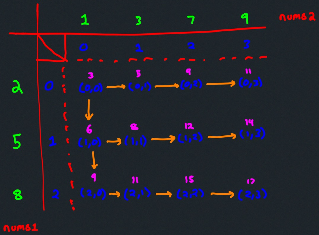
- The illustration above provides an example for the input
nums1 = [2, 5, 8],nums2 = [1, 3, 7, 9]. - The green numbers are from the input arrays themselves while the blue numbers indicate index values — the blue tuples show the index values from each input array.
- The grid is constructed in such a way that it's as if we have an
m x nmatrix withmrows andncolumns (i.e., the number of rows is the same as the number of elements innums1and the number of columns is the same as the number of elements innums2). - The magenta numbers above each tuple show the pair sum for that tuple.
- Suppose a tuple is popped from the heap and processed (e.g., the very first tuple at coordinates
(0,0)). The orange arrows show which tuples are added to the heap after processing the current tuple. Since both input arrays are sorted, note that it only ever makes sense to add tuples to the right of each processed tuple unless the tuple processed is in the first column. This also makes it easy for us to avoid having to keep track of potentially considering duplicate tuples.
LC 632. Smallest Range Covering Elements from K Lists (✓) ★★
You have k lists of sorted integers in non-decreasing order. Find the smallest range that includes at least one number from each of the k lists.
We define the range [a, b] is smaller than range [c, d] if b - a < d - c or a < c if b - a == d - c.
class Solution:
def smallestRange(self, nums: List[List[int]]) -> List[int]:
# initialize a min heap that will contain left boundary candidates
# this min heap will always have k values, one from each list of numbers
left_boundaries = []
for i in range(len(nums)):
nums_arr = nums[i]
heapq.heappush(left_boundaries, (nums_arr[0], i, 0))
# the initial right boundary will be the largest of the left boundary candidates
right = max(triple[0] for triple in left_boundaries)
# initialize the answer to be an infinite interval
ans = [ float('-inf'), float('inf') ]
while left_boundaries:
# minimal left boundary, ith list, jth element
left, i, j = heapq.heappop(left_boundaries)
# only update if strictly tighter range has been found
# (equivalent ranges should not result in an update
# because left boundaries are popped from the min heap
# which means the current answer's left boundary would be smaller)
if right - left < ans[1] - ans[0]:
ans = [left, right]
# only return the answer as soon as one of the k lists has been exhausted
# if we continued despite the condition below, then our range would potentially
# not include an element from each of the k lists
if j + 1 == len(nums[i]):
return ans
# if the condition above was not met, then update the right boundary
# to be the maximum of the current right boundary and the newest added element
right = max(right, nums[i][j + 1])
# the first line of the while loop resulted in removing from the heap
# the jth element from list i; we now add the (j + 1)st element from list i
# to the heap (this ensures the heap still contains an element from each list)
heapq.heappush(left_boundaries, (nums[i][j + 1], i, j + 1))
The solution above, based on the top-voted one on LeetCode, takes some real ingenuity to conjure up. It's a real head-scratcher at first.
As noted in one of the comments on the linked solution above:
The key insight/ intuition (non-obvious) is that the heap always contains ONLY 1 element from each list/ row array. The heap NEVER contains 2 or more elements from the SAME list. This is important because it means that the range calculated at every iteration is always guaranteed to be a range that has exactly 1 element from every single list!
For example, suppose we have the input array from the first example in the problem description on LeetCode:
nums = [[4,10,15,24,26],[0,9,12,20],[5,18,22,30]]
Now add the print statement print(left_boundaries) directly under the beginning of the while loop in the solution above:
[(0, 1, 0), (4, 0, 0), (5, 2, 0)]
[(4, 0, 0), (5, 2, 0), (9, 1, 1)]
[(5, 2, 0), (9, 1, 1), (10, 0, 1)]
[(9, 1, 1), (10, 0, 1), (18, 2, 1)]
[(10, 0, 1), (18, 2, 1), (12, 1, 2)]
[(12, 1, 2), (18, 2, 1), (15, 0, 2)]
[(15, 0, 2), (18, 2, 1), (20, 1, 3)]
[(18, 2, 1), (20, 1, 3), (24, 0, 3)]
[(20, 1, 3), (24, 0, 3), (22, 2, 2)]
The middle number in each tuple denotes which list the left boundary (leftmost tuple number) came from. Note how every time we print the contents of the heap we see that each list (0, 1, and 2 for the example input comprised of three lists) is represented and is only represented once. This is a brilliant way of ensuring an element from each list is always present for each range query.
Initialize heap in O(n) time
Remarks
-
Min heap: Sometimes it is helpful to initialize our own min heap in such a way that we simply append the smallest elements to a list, one at a time. Time and space: .
-
Max heap: Python uses a min heap. Hence, we need to add the biggest elements to the heap, in order, but negate them as we do so. Time and space .
-
Heapify (to min heap): Both approaches above assume we have the luxury of being able to add the minimum or maximum elements to a list and then use that list as a min or max heap, respectively. This is often not the case. We will often want to take an existing list of elements,
arr, and modify it in-place to be a heap in time. This is not a trivial task, as Python's source code for theheapifymethod shows. This is not something we want to have to manually implement ourselves. Fortunately, we don't have to!Simply use Python's
heapifymethod. Time: ; space: . -
Heapify (to max heap): The
heapifyapproach above only applies for a min heap. As noted in this question, Python's source code actually supports a_heapify_maxmethod! But there's not similar support for operations like pushing to the max heap. We effectively have two options to utilize the fulle suite of methods available in Python'sheapqmodule:- Negate the elements of
arrin-place. Then use theheapifymethod to simulate a max heap even though Python is technically maintaining a min heap. Time: ; space: . - Loop through all elements in
arr, negating each along the way, and simultaneously use theheappushmethod to push the element to the max heap we are building. Time: ; space: .
The time cost of the first approach is since the initial loop through to negate all numbers is and the
heapifymethod is also . But practically speaking the second method is also fairly effective and more intuitive. But the first option is surely better for coding interviews! - Negate the elements of
- Min heap
- Max heap
- Heapify (to min heap)
- Heapify (to max heap)
min_heap = []
for i in range(n):
min_heap.append(i)
max_heap = []
for i in range(n - 1, -1, -1):
max_heap.append(-1 * i)
import heapq
arr = [ ... ] # n elements
heapq.heapify(arr)
import heapq
# Approach 1 (negate, heapify in-place); T: O(n); S: O(1)
arr = [ ... ] # n elements
arr = [ -1 * arr[i] for i in range(len(arr)) ] # negate elements in-place
heapq.heapify(arr)
# Approach 2 (negate, build heap); T: O(n lg n); S: O(n)
arr = [ ... ] # n elements
the_heap = []
for num in arr:
heapq.heappush(the_heap, -1 * num)
Examples
LC 1845. Seat Reservation Manager
Design a system that manages the reservation state of n seats that are numbered from 1 to n.
Implement the SeatManager class:
SeatManager(int n)Initializes aSeatManagerobject that will managenseats numbered from1ton. All seats are initially available.int reserve()Fetches the smallest-numbered unreserved seat, reserves it, and returns its number.void unreserve(int seatNumber)Unreserves the seat with the givenseatNumber.
class SeatManager:
def __init__(self, n: int):
self.available = [ i for i in range(1, n + 1) ]
def reserve(self) -> int:
return heapq.heappop(self.available)
def unreserve(self, seatNumber: int) -> None:
heapq.heappush(self.available, seatNumber)
This is an easy problem to over-complicate. It's tempting to craft a solution where we're actively tracking the available and unavailable seats:
class SeatManager:
def __init__(self, n: int):
self.available = [ i for i in range(1, n + 1) ]
self.unavailable = set()
def reserve(self) -> int:
while self.available[0] in self.unavailable:
heapq.heappop(self.available)
seat_number = heapq.heappop(self.available)
self.unavailable.add(seat_number)
return seat_number
def unreserve(self, seatNumber: int) -> None:
self.unavailable.remove(seatNumber)
heapq.heappush(self.available, seatNumber)
But this is really a waste of time and space. The reality is that if we start with a min heap that represents all available seats, then every time we reserve a seat, that seat simply gets popped from the min heap and is no longer an available seat. When we unreserve a seat, that simply means we add the seat back to the heap. The takeaway: there's no need to explicitly track unavailable seats.
Linked lists
What does it mean for two linked list nodes to be "equal"?
TLDR: The default comparison is made by determining whether or not the two nodes point to the same object in memory; that is, node1 == node2 effectively equates to id(node1) == id(node2) by default in Python.
If node1 and node2 are both nodes from a linked list, then what does node1 == node2 actually test? How is the returned boolean computed? The following snippet is illustrative:
nodeA = ListNode(1)
nodeB = nodeA
nodeC = ListNode(1)
print(nodeA == nodeB) # True
print(nodeA == nodeC) # False
As noted on Stack Overflow, for an arbitrary object, the == operator will only return true if the two objects are the same object (i.e., if they refer to the same address in memory). This is often what we actually want when it comes to linked list nodes.
The Python docs about value comparisons back up the note above:
The operators
<,>,==,>=,<=, and!=compare the values of two objects. The objects do not need to have the same type.Chapter Objects, values and types states that objects have a value (in addition to type and identity). The value of an object is a rather abstract notion in Python: For example, there is no canonical access method for an object's value. Also, there is no requirement that the value of an object should be constructed in a particular way, e.g. comprised of all its data attributes. Comparison operators implement a particular notion of what the value of an object is. One can think of them as defining the value of an object indirectly, by means of their comparison implementation.
Because all types are (direct or indirect) subtypes of object, they inherit the default comparison behavior from object. Types can customize their comparison behavior by implementing rich comparison methods like
__lt__(), described in Basic customization.The default behavior for equality comparison (
==and!=) is based on the identity of the objects. Hence, equality comparison of instances with the same identity results in equality, and equality comparison of instances with different identities results in inequality. A motivation for this default behavior is the desire that all objects should be reflexive (i.e.x is yimpliesx == y).
One can override the default __eq__, if desired, but this will likely lead to undesired behavior, particularly in this context of dealing with linked lists. As the Python docs note:
By default,
objectimplements__eq__()by usingis, returningNotImplementedin the case of a false comparison:True if x is y else NotImplemented. For__ne__(), by default it delegates to__eq__()and inverts the result unless it isNotImplemented. There are no other implied relationships among the comparison operators or default implementations; for example, the truth of (x<yorx==y) does not implyx<=y. To automatically generate ordering operations from a single root operation, seefunctools.total_ordering().
What are sentinel nodes and how can they be useful for solving linked list problems?
TLDR: Sentinel or "dummy" nodes can simplify linked list operations, especially those involving the head for singly linked lists (one sentinel node) or the head and tail for doubly linked lists (two sentinel nodes).
Sentinel nodes, also known as "dummy" nodes, often simplify linked list operations considerably, especially when dealing with addition or removal operations involving the head of a linked list. The following brief explanation/definition from ChatGPT is arguably more readable than the linked Wiki article above:
A sentinel node is a dummy or placeholder node used in data structures to simplify boundary conditions and operations. In the context of linked lists, a sentinel node acts as a non-data-bearing head or tail node, eliminating the need for handling special cases for operations at the beginning or end of the list, such as insertions or deletions. It streamlines code by providing a consistent starting or ending point, regardless of whether the list is empty or contains elements.
In the context of solving LeetCode problems (or algorithmic problems in general), you will often see a sentinel node used for singly linked lists in the following manner:
class Solution:
def fn(self, head: Optional[ListNode]) -> Optional[ListNode]:
sentinel = ListNode(-1)
sentinel.next = head
prev = sentinel
curr = head
# do something with prev, curr, and execute other logic
return sentinel.next # return the new/original head of the modified linked list
A very simple example that highlights the utility of sentinel nodes is the following: Given an integer array nums, how can you convert the array into a linked list? The immediate problem that confronts is what to do about the head for the new linked list. It will obviously be the first element in nums, but is there a nice way of building the list? A simple sentinel node allows us to do just that:
def linked_list_from_arr(nums):
sentinel = ListNode(-1)
curr = sentinel
for num in nums:
curr.next = ListNode(num)
curr = curr.next
return sentinel.next
Pointer manipulation and memory indexes
TLDR: Linked list problems are all about pointer manipulation. Rarely do we change val attributes for nodes in a linked list, but we regularly shift nodes around by artfully manipulating next attributes for various nodes (i.e., pointer manipulation).
- Note 1: The assignment
my_var = some_nodemeansmy_varwill always point to the originalsome_nodeobject in memory unless modified directly (e.g.,my_var = something_else). Caveat to this is the note below. - Note 2: The attribute values of
some_node, namelyvalandnext, can be modified indirectly by various means. Hence, even thoughmy_varmay not point to a different object in memory, if the attribute values of the underlying object in memory are changed, then it will likely appear as thoughmy_varno longer refers to its originally referenced object even though it technically does.
Note 1 (variables remain at nodes unless modifed directly):
When you assign a pointer to an existing linked list node, the pointer refers to the object in memory. Suppose you have a node head:
ptr = head
head = head.next
head = None
After these lines of code, ptr still refers to the original head node, even though the head variable changed. This underscores an important concept concerning linked lists and pointer manipulation: variables remain at nodes unless they are modified directly (i.e., ptr = something is the only way to modify ptr).
We can see this more easily and explicitly in Python by using the id() function, which returns the address of the object in memory (for the CPython implementation of Python):
class ListNode:
def __init__(self, val):
self.val = val
self.next = None
one = ListNode(1)
two = ListNode(2)
one.next = two
head = one
print(id(head)) # 4423470576
ptr = head
print(id(ptr)) # 4423470576
head = head.next
print(id(head)) # 4423470480
head = None
print(id(head)) # 4420398192
print(id(ptr)) # 4423470576
Objects are mutable in Python. When we make the assignment ptr = head, we are effectively making ptr point to the same memory address as head. The assignment more or less looks like the following:
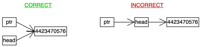
Subsequently, when we assign head to head.next, we are making head point to the same memory address as head.next:
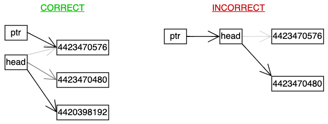
Note that ptr is not still pointing at head (it's pointing to the object in memory that head originally pointed to). The takeaway: a variable that serves as a specific node assignment will remain as such a specific node assignment unless modified directly to point to another node. This is what allows us above to point ptr to head and then do whatever we want to with head all while maintaining our reference to the original head with ptr.
Note 2 (node attributes such as val and next may be modified indirectly):
As detailed in the note above, the code block
ptr = head
head = head.next
head = None
means that ptr, unless modified directly, will always point to the object in memory originally referred to by head.
Importantly, however, the object in memory originally referred to by head can have its attributes modified indirectly (i.e., the val and next attributes of the head object to which ptr points can be modified without altering ptr directly). The following example can help illustrate this important observation:
head = ListNode(100)
node1 = ListNode(1)
node2 = ListNode(2)
node3 = ListNode(3)
head.next = node1
node1.next = node2
node2.next = node3
sentinel = ListNode(-1)
sentinel.next = head
ptr = head
head = head.next
head = None
print(id(ptr)) # 0123456789
print(ptr) # 100 -> 1 -> 2 -> 3 -> None
print(ptr.val) # 100
print(ptr.next) # 1 -> 2 -> 3 -> None
sentinel.next.val = 7 # original "head" attribute "val" changes from 100 to 7
sentinel.next.next = node2 # original "head" attribute "next" changes from node1 to node2
print(id(ptr)) # 0123456789
print(ptr) # 7 -> 2 -> 3 -> None
print(ptr.val) # 7
print(ptr.next) # 2 -> 3 -> None
Note that ptr was never modified directly and that it still points to the same object in memory before and after the sentinel.next.[val|next] changes (i.e., printing id(ptr) before and after the changes confirms this since the printed values are the same).
But it certainly seems like ptr has changed somehow. This is because the object ptr points to has changed in terms of its val and next attribute values. We changed those values indirectly by altering sentinel.next, which pointed to the same mutable object in memory as ptr. Altering the attribute values of the original head object in memory directly with ptr.[val|next] or indirectly with sentinel.next.[val|next] makes no difference. The effect is the same: ptr looks different even though it still points to the same object in memory.
Example: A solution to problem LC 2095. Delete the Middle Node of a Linked List can illustrate the concepts in the second note in a concrete, practical manner:
class Solution:
def deleteMiddle(self, head: Optional[ListNode]) -> Optional[ListNode]:
sentinel = ListNode(-1)
sentinel.next = head
prev = sentinel
slow = head
fast = head
# slow points to middle node upon termination
while fast and fast.next:
prev = slow
slow = slow.next
fast = fast.next.next
# skip middle node, effectively removing it
prev.next = prev.next.next
return sentinel.next
How does this illustrate the utility of the second note? Consider the case where the linked list is just a single node: [1]. Removing the middle node means removing the only node, meaning we should return [] or None. How is the solution above correct for this edge case since the while loop does not fire, sentinel.next originally points to head, and we ultimately return sentinel.next without ever making a direct reassignment? How does sentinel.next end up pointing to a null value even though it originally points to head?
The reason is due to how prev is being manipulated. Since prev points to sentinel and the while loop doesn't fire, the assignment prev.next = prev.next.next effectively changes what sentinel.next points to; that is, we're not changing sentinel directly, but we are changing the next attribute value of the underlying object in memory being pointed to by sentinel. Hence, prev.next = prev.next.next is effectively the assignment sentinel.next = sentinel.next.next; since sentinel.next points to head and head.next is None, we get our desired result by returning the null value (which indicates the single object has been removed).
Visualizing singly linked lists and debugging your code locally
TLDR: Add a simple __repr__ method to the base ListNode class. This lets you view the linked list extending from any given my_node by simply running print(my_node). To effectively use sample LeetCode inputs in your local testing, you'll need a function arr_to_ll to convert integer arrays into linked lists.
Linked list problems are all about pointer manipulation and it can help a ton to see things, especially if you need to debug issues with your code. LeetCode almost always provides a linked list by simply providing the head node, where all nodes in the list have been created with the following ListNode class (or some minor variation):
class ListNode:
def __init__(self, x):
self.val = x
self.next = None
Given any node, probably the easiest way to visualize the singly linked list that extends from this node is to implement a basic __repr__ method as part of the ListNode class:
class ListNode:
def __init__(self, x):
self.val = x
self.next = None
def __repr__(self):
node = self
nodes = []
while node:
nodes.append(str(node.val))
node = node.next
nodes.append('None')
return ' -> '.join(nodes)
Of course, LeetCode generally shows a linked list as input by providing an integer array. To effectively test your local code on LeetCode inputs, it's necessary to first convert the integer array to a linked list:
def arr_to_ll(arr):
sentinel = ListNode(-1)
curr = sentinel
for val in arr:
new_node = ListNode(val)
curr.next = new_node
curr = curr.next
return sentinel.next
We can now effectively use LeetCode inputs, visualize them, and also subsequently visualize whatever changes we make to the input:
example_input = [5,2,6,3,9,1,7,3,8,4]
head = arr_to_ll(example_input)
print(head) # 5 -> 2 -> 6 -> 3 -> 9 -> 1 -> 7 -> 3 -> 8 -> 4 -> None
Fast and slow pointers
Remarks
The "fast and slow" pointer technique is a two pointer technique with its own special use cases when it comes to linked lists. Specifically, the idea is that the pointers do not move side by side — they could move at different "speeds" during iteration, begin iteration from different locations, etc. Whatever the abstract difference is, the important point is that they do not move side by side in unison.
There are many two pointer variations when it comes to arrays and strings, but the fast and slow pointer technique for linked lists usually presents itself as, "move the slow pointer one node per iteration, and move the fast node two nodes per iteration."
def fn(head):
slow = head
fast = head
ans = 0
while fast and fast.next:
# some logic
slow = slow.next
fast = fast.next.next
return ans
Examples
Return the middle node value of a linked list with an odd number of nodes (✓)
def get_middle(head):
slow = head
fast = head
while fast and fast.next:
slow = slow.next
fast = fast.next.next
return slow.val
Time: . We linearly process the entire linked list.
Space: . Additional memory used does not scale with input.
The main problem here is not knowing the length of the linked list ahead of time. We could push the node values into an array and then find the middle node value that way, but that would be cheating and would never pass in an interview. We could also iterate through the entire linked list, note the full length, iterate through half the full length, and then report the value of the middle node. But that also seems potentially inefficient.
The solution above takes advantage of the fact that the slow node will have traveled half the distance of the fast node once the while loop terminates (meaning the slow node will be in the middle of the list, as desired). We have to be more careful if the number of nodes can be odd or even, but this problem stipulates we have an odd number of nodes.
It's easier to see with a visualization like the following (x is the desired node while s and f denote the slow and fast pointers, respectively):
x
12345
s
f
x
12345
s
f
x
12345
s
f
Note that now fast is not null, but fast.next is null, meaning the while loop will not execute, and s points to the middle node, x, as desired.
Return the kth node from the end provided that it exists (✓)
def find_node(head, k):
slow = head
fast = head
for _ in range(k):
fast = fast.next
while fast:
slow = slow.next
fast = fast.next
return slow
Time: . The entire list is processed.
Space: . No additional memory is consumed as the input scales.
The idea here is to first advance the fast pointer k units ahead of the slow pointer and then to move them at the same speed for each iteration, meaning they will always be k units apart. When the fast pointer reaches the end (i.e., it points to null), the slow pointer will still be k nodes behind the fast pointer, which is the desired result.
The following illustration, where k = 3, may help:
k
1234567
s
f
k
1234567
s
f
k
1234567
s
f
k
1234567
s
f
k
1234567
s
f
k
1234567
s
f
LC 141. Linked List Cycle (✓) ★
Given head, the head of a linked list, determine if the linked list has a cycle in it.
There is a cycle in a linked list if there is some node in the list that can be reached again by continuously following the next pointer. Internally, pos is used to denote the index of the node that tail's next pointer is connected to. Note that pos is not passed as a parameter.
Return true if there is a cycle in the linked list. Otherwise, return false.
class Solution:
def hasCycle(self, head: Optional[ListNode]) -> bool:
slow = head
fast = head
while fast and fast.next:
slow = slow.next
fast = fast.next.next
if slow == fast:
return True
return False
Time: . The worst-case scenario is if there is a cycle and the slow pointer enters the cycle right after the fast pointer has passed the starting point of the cycle, meaning the fast pointer must travel the entire distance of the cycle again before catching the slow pointer. Regardless, the time cost is .
Space: . Additional memory is not consumed as the input scales.
The placement of the
if slow == fast:
return True
block in the solution above is important: if we did it before moving the pointers, then we would trivially return True every time by virtue of the fact that slow == fast == head at the outset.
TLDR of Floyd's cycle-detection algorithm
Intuitively, we need to think about how slow and fast can relate to each other within the cycle (if one exists). If they meet at the beginning of the cycle (pos in the problem description), then great! We're done. If not, we need to consider how fast can catch up to slow. It clearly will, but the question is whether or not it might somehow skip it. It won't. The illustration below, where x denotes where fast (f) and slow (s) will meet, explains why (assume fast is close to slow now, either 1 node back or 2):
# `fast` is 1 node behind `slow` (a single iteration is needed for `fast` to catch `slow`)
## start:
f s x
_ _ _ _ _ _
## after iteration 1:
f
s
x
_ _ _ _ _ _
# `fast` is 2 nodes behind `slow` (two iterations are needed for `fast` to catch `slow`)
## start:
f s x
_ _ _ _ _ _
## after iteration 1:
f s x
_ _ _ _ _ _
## after iteration 2:
f
s
x
_ _ _ _ _ _
The solution above takes advantage of Floyd's cycle-detection algorithm, which is quite overcomplicated on the Wikipedia link. The main outcome of the algorithm is that the slow and fast pointers above must be equal at some point if there is a cycle. But how do we know this to be true? Would it be possible for the fast pointer to "jump" the slow pointer in some way? How do we know they'll actually meet if there's a cycle?
The easiest way to answer this question is to break down all of the possibilities once slow and fast are both within the cycle; that is, fast will obviously be well ahead of slow until slow actually enters the cycle, at which point slow and fast will either be at the same node or fast will be behind slow. We have the following possibilities:
- Case 1:
fastandslowmeet exactly whenslowenters the cycle (i.e., at the beginning of the cycle) - Case 2:
fastis exactly one node behindslow, and the two nodes will meet on the very next iteration sinceslowwill move forward one node andfastwill move forward two nodes - Case 3:
fastis exactly two nodes behindslow, and the nodes will meet after two more iterations sinceslowwill have moved two more nodes andfastwill have moved four more nodes - Case 4:
fastis more than two nodes behindslow, which meansfastwill eventually catch up toslowin such a way that this case resolves into either case 2 or case 3, which means the nodes will still meet
The important takeaway above is that fast will never jump slow. The two nodes must meet if there is a cycle.
It's worth mentioning that we can also implement a solution that uses a hash set:
class Solution:
def hasCycle(self, head: Optional[ListNode]) -> bool:
seen = set()
while head:
if head in seen:
return True
seen.add(head)
head = head.next
return False
But this is less efficient than the original solution since it uses space instead of .
LC 876. Middle of the Linked List (✓)
Given a non-empty, singly linked list with head node head, return a middle node of linked list.
If there are two middle nodes, return the second middle node.
class Solution:
def middleNode(self, head: Optional[ListNode]) -> Optional[ListNode]:
slow = head
fast = head
while fast and fast.next:
slow = slow.next
fast = fast.next.next
return slow
Time: . The entire list is processed.
Space: . Memory consumed does not increase as the input scales.
This uses the classic fast-slow technique. For an odd-length list:
x
12345
s
f
x
12345
s
f
x
12345
s
f
Done! And we're fortunate for even-length lists since we're asked to return the second middle node:
x
123456
s
f
x
123456
s
f
x
123456
s
f
x
123456
s
f
Things work out nicely in this case.
What if, however, we were asked to return the first middle node? Then we could make use of a prev pointer to basically lag behind the slow pointer. Which node we returned at the end would depend on where fast was (not null for odd-length lists and null for even-length lists):
class Solution:
def middleNode(self, head: Optional[ListNode]) -> Optional[ListNode]:
slow = head
fast = head
while fast and fast.next:
prev = slow
slow = slow.next
fast = fast.next.next
return prev if not fast else slow
LC 142. Linked List Cycle II (✓) ★★
Given a linked list, return the node where the cycle begins. If there is no cycle, return null.
There is a cycle in a linked list if there is some node in the list that can be reached again by continuously following the next pointer. Internally, pos is used to denote the index of the node that tail's next pointer is connected to. Note that pos is not passed as a parameter.
Notice that you should not modify the linked list.
class Solution:
def detectCycle(self, head: Optional[ListNode]) -> Optional[ListNode]:
slow = head
fast = head
while fast and fast.next:
slow = slow.next
fast = fast.next.next
if slow == fast:
slow = head
while slow != fast:
slow = slow.next
fast = fast.next
return slow
return None
Determining whether or not a cycle exists is a pre-requisite for coming up with a solution for this problem. We can effectively tweak our solution to LC 141. Linked List Cycle in order to come up with the solution above:
class Solution:
def hasCycle(self, head: Optional[ListNode]) -> bool:
slow = head
fast = head
while fast and fast.next:
slow = slow.next
fast = fast.next.next
if slow == fast:
return True
return False
That is, as the highlighted lines above suggest, we need to do something once we actually have determined that we have a cycle. What should we do? The following image (from this YouTube video) may help:
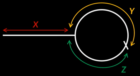
This image shows how X units are traveled before the cycle starts. We'll assume we're moving in a counterclockwise direction once we've entered the cycle. We can't know for sure how many times fast might travel the full cycle of Y + Z units before slow enters the cycle. The important observation is that eventually there will come a revolution where fast starts at the beginning of the cycle and slow joins the cycle during this revolution.
How many units does fast travel before it meets slow? Where exactly fast is when slow enters the cycle does not matter — the important point is that it must travel the full distance of Z + Y + Z before coming back around to meet slow. In total, then, fast travels a distance of X + R(Z + Y) + (Z + Y + Z), where R(Z + Y) denotes that fast has traveled R full cycle lengths before it starts its last revolution before slow enters the cycle. Since slow travels a total distance of X + Z, we have the following useful equation (we discard R(Z + Y) during the second simplifying step due to its cyclical nature):
2(X + Z) = X + R(Z + Y) + (Z + Y + Z)
2X + 2Z = X + 2Z + Y
X = Y
What the above equation means in the context of this problem is that all we really need to do to actually return the node at which the cycle starts is reset one of the nodes to start at the head and then just move them together in unison until they meet again (at the beginning of the cycle). We can then return the desired node.
LC 83. Remove Duplicates from Sorted List (✓) ★
Given the head of a sorted linked list, delete all duplicates such that each element appears only once. Return the linked list sorted as well.
class Solution:
def deleteDuplicates(self, head: Optional[ListNode]) -> Optional[ListNode]:
curr = head
while curr and curr.next:
if curr.val == curr.next.val:
curr.next = curr.next.next
else:
curr = curr.next
return head
Time: . The entire input list is processed in a linear fashion.
Space: . The memory consumed does not increase as the input scales.
The solution above is probably less obvious than it should seem at first glance, but it cleverly avoids the need to use two pointers (slow and fast) because of how curr is manipulated. Three observations worth making:
- It only makes sense to test for duplicates if we have at least two nodes for comparison. Hence, we only look to make modificates while
currandcurr.nextboth exist. - If we have
node1 -> node2 -> ..., then how can we effectively "delete"node2from this list? We do so in the following standard way (i.e., using its previous node,node1, to skip it):node1.next = node1.next.next. Such an assignment meansnode2is "skipped" fromnode1and effectively removed from the chain. In the context of this problem, ifcurr.val == curr.next.val, then we want to removecurr.nextfrom the list, and we do so in the standard way:curr.next = curr.next.next. - If
currand the next node have different values, then we simply advancecurrin the standard way:curr = curr.next. Note howcurris only ever advanced/reassigned when we encounter different values. Since the list is already sorted, this ensures the resultant list only contains distinct values, as desired.
The solution above is elegant, straightforward, and uncomplicated; however, if we wanted to use two pointers, then how would we do so? We could use lag and lead as slow and fast pointers, respectively. The idea is that lag always points to the first non-duplicate value we find, and it "lags" behind lead until lead discovers a value for which lead.val != lag.val, whereby lag.next now points to this new non-duplicate node/value, and we update lag to point to where lead was when this non-duplicated value was discovered.
The main potential "gotcha" with this approach occurs at the end of the list. If there are duplicates at the end of the list, then lag points at the first duplicate value and lead never discovers a non-duplicate value. Thus, if we don't manually make the assignment lag.next = None after lead has iterated through the entire list, then we run the risk of accidentally including all duplicated values at the end of the list.
Here's the working solution for this two pointer approach:
class Solution:
def deleteDuplicates(self, head: Optional[ListNode]) -> Optional[ListNode]:
if not head:
return None
lead = head
lag = head
while lead:
lead = lead.next
if lead and lead.val != lag.val:
lag.next = lead
lag = lead
lag.next = None
return head
The primary difference between the solutions is how the duplicate nodes are being deleted. In the first approach, duplicate nodes are being deleted as they are encountered. A duplicate node is deleted as soon as it's encountered: curr.next = curr.next.next. In the second approach, all duplicate nodes are deleted as soon as a non-duplicate value is found: lag.next = lead.
LC 2095. Delete the Middle Node of a Linked List (✓)
You are given the head of a linked list. Delete the middle node, and return the head of the modified linked list.
The middle node of a linked list of size n is the ⌊n / 2⌋th node from the start using 0-based indexing, where ⌊x⌋ denotes the largest integer less than or equal to x.
- For
n = 1, 2, 3, 4, and5, the middle nodes are0,1,1,2, and2, respectively.
class Solution:
def deleteMiddle(self, head: Optional[ListNode]) -> Optional[ListNode]:
sentinel = ListNode(-1)
sentinel.next = head
prev = sentinel
slow = fast = head
while fast and fast.next:
prev = slow
slow = slow.next
fast = fast.next.next
prev.next = prev.next.next
return sentinel.next
Since slow will point to the middle node after the while loop terminates above, what we really need is for the node prior to slow to skip it, effectively deleting it: prev.next = prev.next.next.
LC 19. Remove Nth Node From End of List (✓)
Given the head of a linked list, remove the nth node from the end of the list and return its head.
Follow up: Could you do this in one pass?
class Solution:
def removeNthFromEnd(self, head: Optional[ListNode], n: int) -> Optional[ListNode]:
sentinel = ListNode(-1)
sentinel.next = head
prev = sentinel
slow = fast = head
for _ in range(n):
fast = fast.next
while fast:
prev = slow
slow = slow.next
fast = fast.next
prev.next = prev.next.next
return sentinel.next
The idea: advance fast nodes past slow so that there are always nodes between these pointers. When the while loop terminates, slow will be units behind fast or nodes from the end of the list, as desired. But we need to delete this node, hence the use of the prev pointer.
LC 82. Remove Duplicates from Sorted List II (✓) ★
Given the head of a sorted linked list, delete all nodes that have duplicate numbers, leaving only distinct numbers from the original list. Return the linked list sorted as well.
class Solution:
def deleteDuplicates(self, head: Optional[ListNode]) -> Optional[ListNode]:
sentinel = ListNode(-1)
sentinel.next = head
prev = sentinel
curr = head
while curr and curr.next:
if curr.val == curr.next.val:
while curr and curr.next and curr.val == curr.next.val:
curr.next = curr.next.next
curr = curr.next
prev.next = curr
else:
prev = curr
curr = curr.next
return sentinel.next
This problem is obviously quite similar to LC 83. Remove Duplicates from Sorted List, but the requirement to remove all numbers that have duplicates basically makes this a completely different problem. As always, it's amazing how helpful a drawing that solves a basic example can be:
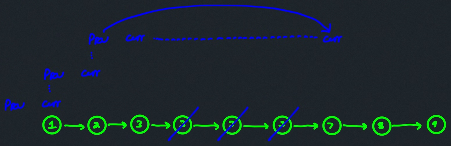
The picture above illustrates how prev and curr need to be moved together in unison when there are not duplicates; however, if duplicates are encountered, then we can employ a strategy similar to that used in LC 83, where we effectively "delete" duplicates as they are encountered by changing the next attribute for curr: curr.next = curr.next.next. The twist with this problem is that we want to retain none of the duplicate values once we've encountered a non-duplicate value. As the figure suggests, one way of achieving this is to move curr past the last duplicate, and then change the next attribute for prev to point to the updated, non-duplicate curr node. This effectively cuts out all duplicate values, and prev itself is only ever updated when non-duplicate values are adjacent.
LC 1721. Swapping Nodes in a Linked List (✓)
You are given the head of a linked list, and an integer k.
Return the head of the linked list after swapping the values of the kth node from the beginning and the kth node from the end (the list is 1-indexed).
class Solution:
def swapNodes(self, head: Optional[ListNode], k: int) -> Optional[ListNode]:
left = right = null_checker = head
for _ in range(k - 1):
left = left.next
null_checker = null_checker.next
while null_checker.next:
right = right.next
null_checker = null_checker.next
left.val, right.val = right.val, left.val
return head
The fast-slow pointer approach above works great for this problem where only the node values need to be swapped. But switching the nodes themselves requires a little bit more work:
class Solution:
def swapNodes(self, head: Optional[ListNode], k: int) -> Optional[ListNode]:
def swap_nodes(prev_left, prev_right):
if not prev_left or not prev_right \
or not prev_left.next or not prev_right.next \
or prev_left.next == prev_right.next:
return
left = prev_left.next
right = prev_right.next
prev_left.next, prev_right.next = right, left
right.next, left.next = left.next, right.next
sentinel = ListNode(-1)
sentinel.next = head
prev_left = prev_right = sentinel
null_checker = head
for _ in range(k - 1):
prev_left = prev_left.next
null_checker = null_checker.next
while null_checker.next:
prev_right = prev_right.next
null_checker = null_checker.next
swap_nodes(prev_left, prev_right)
return sentinel.next
See more about this approach in the "swap two nodes" template section.
Reverse a linked list
Remarks
The template below is the simplest way of reversing a portion of a linked list from a given node (potentially the entire list if given the head of a linked list). One important observation is that the reversed portion is effectively severed from the rest of the list.
For example:
ex = [1,2,3,4,5,6] # integer array
head = arr_to_ll(ex) # convert integer array to linked list
print(fn(head.next.next)) # start reversal from node 3
# outcome: 6 -> 5 -> 4 -> 3 -> None
Suppose the outcome above is not desirable and instead we wanted the reversal to be incorporated into the original list: 1 -> 2 -> 6 -> 5 -> 4 -> 3 -> None. We clearly need to preserve the node previous to the node where the reversal starts (i.e., the 2 node is a sort of "connecting" node that needs to be preserved). Solving this problem is outside the scope of this template; however, the subsequent template for reversing k nodes of a linked list does solve this problem.
def fn(node):
prev = None
curr = node
while curr:
next_node = curr.next
curr.next = prev
prev = curr
curr = next_node
return prev
Examples
LC 206. Reverse Linked List (✓)
Given the head of a singly linked list, reverse the list, and return the reversed list.
class Solution:
def reverseList(self, head: Optional[ListNode]) -> Optional[ListNode]:
prev = None
curr = head
while curr:
next_node = curr.next # ensure we don't lost the connection to the next node when we reverse the direction of the pointer
curr.next = prev # reverse the direction of the pointer
prev = curr # update `prev` to be `curr` in preparation for the next node to be processed
curr = next_node # move forward in the iteration to process the remainder of the list
return prev
Time: . The entire list is processed in a linear fashion.
Space: . Memory consumed does not increase as input scales.
This is a classic linked list "pointer manipulation" problem, and the approach above is the conventionally efficient approach, where next_node effectively serves as a temporary variable (so we don't lose the linked list connection when we make the assignment curr.next = prev).
One thing worth noting about this conventional approach is how the reversed segment is effectively broken off from the rest of the list if the reversal is started on a node other than the linked list's head. For example, consider the list 1 -> 2 -> 3 -> 4 -> 5 -> None. If we start the reversal at node 3, then reversing 3 -> 4 -> 5 gives us 5 -> 4 -> 3, but what happens to the rest of the list? We lose the connection. Hence, starting from the head of the original linked list we have 1 -> 2 -> 3 -> None while starting from the head of the reversed segment gives us 5 -> 4 -> 3 -> None.
Python's support for tuple packing/unpacking and multiple assignment means we can simplify the reversal in a pretty dramatic fashion:
class Solution:
def reverseList(self, head: Optional[ListNode]) -> Optional[ListNode]:
prev = None
curr = head
while curr:
curr.next, prev, curr = prev, curr, curr.next
return prev
Here's a quick breakdown:
- Tuple Packing: The expression on the right side of the assignment,
prev, curr, curr.next, effectively creates a tuple of these three references/values. This happens before any assignments are made, which means the original values are preserved in the tuple. - Multiple Assignment: The left-hand side of the assignment has three variables,
curr.next, prev, curr, awaiting new values. Python will assign the values from the tuple on the right-hand side to these variables in a left-to-right sequence. - Tuple Unpacking: The assignment unpacks the values stored in the tuple into the variables on the left. This happens simultaneously, so the operations do not interfere with each other. Specifically:
curr.nextis assignedprev. This reverses the pointer/link of the current node to point to the previous node, effectively starting the reversal of the linked list.previs assignedcurr. This moves theprevpointer one node forward to the current node, which after the assignment, becomes the new "previous" node.curris assignedcurr.next(the originalcurr.nextbefore any changes). This moves thecurrpointer one node forward in the original list, to continue the reversal process on the next iteration.
The one-liner above is slick and may be useful for problems where reversing the linked list (or part of it) is naturally part of the solution (e.g., LC 2130. Maximum Twin Sum of a Linked List).
LC 24. Swap Nodes in Pairs (✓) ★★
Given a linked list, swap every two adjacent nodes and return its head.
class Solution:
def swapPairs(self, head: Optional[ListNode]) -> Optional[ListNode]:
sentinel = ListNode(-1)
sentinel.next = head
prev = sentinel
left = head
while left and left.next:
right = left.next # identify the right node in the left-right pair to be swapped
next_left = left.next.next # ensure the connection is not lost when reversing the `right` pointer
right.next = left # reverse the `right` pointer to point at the `left` node
left.next = next_left # point the `left` node to the preserved connection beyond the `right` node
prev.next = right # maintain pointer connections to ensure continuity after swap
prev = left # move `prev` forward in preparation for next pair to be processed
left = next_left # move `left` forward in preparation for next pair to be processed
return sentinel.next
Time: . The entire list is processed in a linear fashion.
Space: . Memory consumed does not increase as input size scales.
As with most linked list problems, this problem becomes much easier if we take a moment to draw what happens for a general pair swap (the orange arrows indicate changes to each node's next attribute):
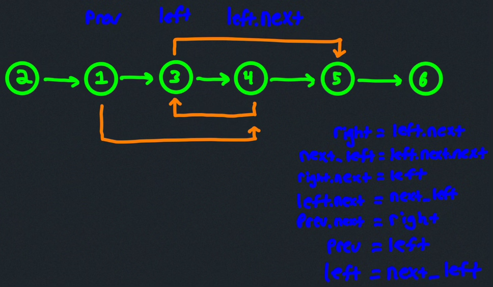
The solution above naturally presents itself from this figure.
It's worth reflecting on why prev is necessary in the solution above. Consider what would happen in the previous figure if prev were not present — what would happen after swapping 3 and 4? The connections would get mangled — we'd have 4 -> 3 as desired, but without prev we'd end up having 1 -> 3 after the swap, which is not desired. We need to maintain the connections to ensure continuity is preserved after each swap is made, and this is easiest to do with a prev pointer, as above.
That's the entire purpose of the prev pointer in the solution above — it's used to ensure proper connections are maintained after swaps.
LC 2130. Maximum Twin Sum of a Linked List (✓) ★★
In a linked list of size n, where n is even, the ith node (0-indexed) of the linked list is known as the twin of the (n-1-i)th node, if 0 <= i <= (n / 2) - 1.
- For example, if
n = 4, then node0is the twin of node3, and node1is the twin of node2. These are the only nodes with twins forn = 4.
The twin sum is defined as the sum of a node and its twin.
Given the head of a linked list with even length, return the maximum twin sum of the linked list.
class Solution:
def pairSum(self, head: Optional[ListNode]) -> int:
def reverse(node):
prev = None
curr = node
while curr:
next_node = curr.next
curr.next = prev
prev = curr
curr = next_node
return prev
slow = fast = head
while fast and fast.next:
slow = slow.next
fast = fast.next.next
left = head
right = reverse(slow)
ans = 0
while right:
ans = max(ans, left.val + right.val)
left = left.next
right = right.next
return ans
Time: . We process the entire list in a linear fashion.
Space: . Memory consumed does not increase as the input size scales.
This is a fun one: Find the middle of the linked list, reverse the rest of the linked list, and then iterate back towards the middle from the head as well as from the end that was just reversed (i.e., the head of the newly reversed portion of the linked list), maintaining the maximum pairwise sum as you go.
Small potential "gotcha": after the reversal, slow points to the second middle node of the linked list (since the total number of nodes is always even), which means it's a single node past what we need to iterate through on the left hand side. The last while loop condition needs to be while right; otherwise, if we used while left, then trying to access right.val would eventually throw an error because the reversed segment on the right would be exhausted while there's a single node left on the left side.
LC 234. Palindrome Linked List (✓)
Given the head of a singly linked list, return true if it is a palindrome.
class Solution:
def isPalindrome(self, head: Optional[ListNode]) -> bool:
def reverse(node):
prev = None
curr = node
while curr:
next_node = curr.next
curr.next = prev
prev = curr
curr = next_node
return prev
if not head or not head.next:
return True
slow = fast = head
while fast and fast.next:
slow = slow.next
fast = fast.next.next
left = head
right = reverse(slow)
while right:
if left.val != right.val:
return False
left = left.next
right = right.next
return True
The solution above is likely the intended solution for this problem even though destroying the original linked list is not a very desirable side effect. It's also nice that we do not have to consider the length of the list when making the reversal. An odd-length list like 1 -> 2 -> 3 -> 2 -> 1 means that once the reversal occurs we get 1 -> 2 -> 3 starting from the original head and 1 -> 2 -> 3 starting from the head of the reversed segment. An even-length list like 1 -> 2 -> 2 -> 1 means after the reversal we have 1 -> 2 -> 2 starting from the head of the original list and 1 -> 2 starting from the head of the reversed segment. This is why it's important that our last while loop uses the condition while right as opposed to while left.
If the side effect mentioned above is not allowed, then we can use the "reverse k nodes in-place" template to determine whether or not the list's values are palindromic and also restore the list itself (although the logic becomes a bit more complicated):
class Solution:
def isPalindrome(self, head: Optional[ListNode]) -> bool:
def reverse_k_nodes(prev, k):
if not prev.next or k < 2:
return prev.next
rev_start = prev.next
next_node = rev_start.next
rev_end = rev_start
count = 1
while count <= k - 1 and next_node:
rev_start.next = next_node.next
next_node.next = prev.next
prev.next = next_node
next_node = rev_start.next
count += 1
return rev_end
if not head or not head.next:
return True
sentinel = ListNode(-1)
sentinel.next = head
prev = sentinel
slow = fast = head
char_count = 1
while fast and fast.next:
prev = slow
slow = slow.next
fast = fast.next.next
char_count += 1
middle = slow if fast else prev
reverse_k_nodes(middle, char_count)
right = middle.next
left = head
for _ in range(char_count - 1):
if left.val != right.val:
reverse_k_nodes(middle, char_count)
return False
left = left.next
right = right.next
# this reversal optional since values are palindromic after the in-place reversal
reverse_k_nodes(middle, char_count)
return True
LC 2487. Remove Nodes From Linked List★★
You are given the head of a linked list.
Remove every node which has a node with a strictly greater value anywhere to the right side of it.
Return the head of the modified linked list.
class Solution:
def removeNodes(self, head: Optional[ListNode]) -> Optional[ListNode]:
def reverse(node):
prev = None
curr = node
while curr:
curr.next, prev, curr = prev, curr, curr.next
return prev
rev_head = reverse(head)
sentinel = ListNode(float('-inf'))
sentinel.next = rev_head
prev = sentinel
curr = rev_head
while curr:
if prev.val > curr.val:
prev.next = curr.next
else:
prev = curr
curr = curr.next
return reverse(sentinel.next)
The issue at the beginning of the problem lies in how the pointers restrict how we can manage what happens with decreasing values. Reversing the linked list as a pre-processing step is an effective strategy here. Then we can simply adjust pointers as needed to ensure our linked list is weakly increasing. Then as a final step we return the reversal of that linked list.
LC 2816. Double a Number Represented as a Linked List (✓)
You are given the head of a non-empty linked list representing a non-negative integer without leading zeroes.
Return the head of the linked list after doubling it.
class Solution:
def doubleIt(self, head: Optional[ListNode]) -> Optional[ListNode]:
def reverse(node):
prev = None
curr = node
while curr:
curr.next, prev, curr = prev, curr, curr.next
return prev
rev_head = reverse(head)
carried = 0
sentinel = ListNode(-1)
sentinel.next = rev_head
curr = sentinel.next
while curr:
doubled = carried + curr.val * 2
new_val = doubled % 10
carried = doubled // 10
curr.val = new_val
curr = curr.next
doubled_head = reverse(sentinel.next)
if carried:
new_head = ListNode(carried)
new_head.next = doubled_head
return new_head
else:
return doubled_head
The basic idea above is to first reverse the list so we can more easily manage the updating of node values — values range from 0 through 9 which means the doubled values range from 0 through 18, where the original value being 5 or more means having a doubled value in the range 10-18, which requires carrying.
We perform the needed value updates and maintain the number being carried along the way. Once we're done, we reverse the new list. If carried is 0, then we're done, but if carried is not 0, then whatever carried is should become the first value in our new list.
The editorial for this problem is great. Reversing twice as done above is not necessary even though it is sufficient. There's a really slick one-pointer approach that takes advantage of how "carrying" works in terms of whether or not we ever need to update a node's value.
Reverse k nodes of a linked list in-place
What is the purpose of this template?
The purpose of the template, of course, is to reverse k nodes of a linked list in-place. But, as this post notes (the post that originally motivated this template), the template below does not break off the section to be reversed (this is what happens with the conventional reversal, as detailed in the previous template).
The template below leaves the start node of the section linked to the rest of the list and moves the remaining nodes one by one to the front. This results in the k-length section (starting at the start node) being reversed, the original start node being the end node of the reversed section, and the original start node being connected to the rest of the list instead of being severed or pointing to None. The next remark provides some intuition as to how this actually works.
What is the intuition behind how and why this template works?
The core idea is actually somewhat simple: given a prev node that precedes the start node for the k-length section to be reversed, we effectively move the k - 1 nodes that follow the start so that they now come before the start node. One at a time. Suppose we want the section 3 -> 4 -> 5 -> 6 to be reversed in the following list (spaces added to emphasize section being reversed):
1 -> 2 -> 3 -> 4 -> 5 -> 6 -> 7 -> 8 -> 9 -> None
The desired outcome would then be the following list:
1 -> 2 -> 6 -> 5 -> 4 -> 3 -> 7 -> 8 -> 9 -> None
Above, we see that k = 4, prev is node 2, and node 3 is the start of the section to be reversed. Our template stipulates that nodes 4, 5, 6, which originally follow node 3, will now be moved to come before node 3. One at a time:
1 -> 2 -> 3 -> 4 -> 5 -> 6 -> 7 -> 8 -> 9 -> None # start
1 -> 2 -> 4 -> 3 -> 5 -> 6 -> 7 -> 8 -> 9 -> None # after iteration 1
1 -> 2 -> 5 -> 4 -> 3 -> 6 -> 7 -> 8 -> 9 -> None # after iteration 2
1 -> 2 -> 6 -> 5 -> 4 -> 3 -> 7 -> 8 -> 9 -> None # after iteration 3
Hence, k - 1 iterations are needed to reverse the k-length section in-place, and we conclude by returning the end node for the reversed section, node 3 in this case. Here's a more colorful illustration of what things look like for each iteration:
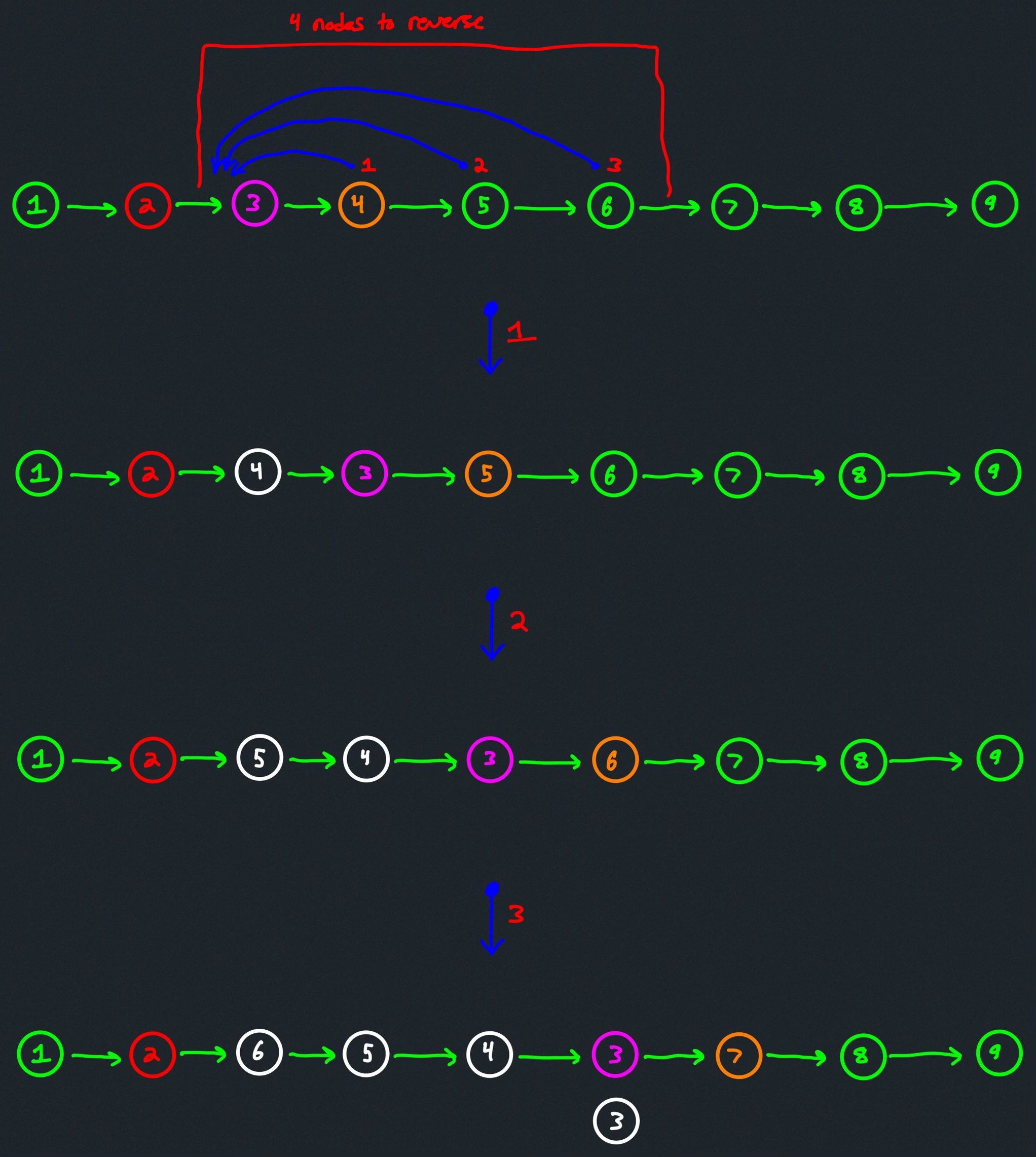
The top part of the image shows the initial list and which four nodes need to be reversed, where the red numbering 1, 2, and 3 indicates where the nodes end up after that many iterations have taken place. The actual node coloring scheme:
- Red
2: This fixed node denotes the node preceding where the reversal starts. - Magenta
3: This fixed coloring denotes the node where the reversal starts (and also the node returned at the end). - Orange nodes: The orange node is always the "next node" to be moved to the front (i.e.,
next_nodein the template). - White nodes: This coloring indicates the nodes that have already been processed. The last iteration shows how the node where the reversal started concludes with its proper positioning at the end of the reversed segment.
The image above, particularly the top part of the image with the initial list and the arrow indicators which show how each node moves for each iteration, provides an intuition for how and why the template works. The following image shows the mechanics in more detail:
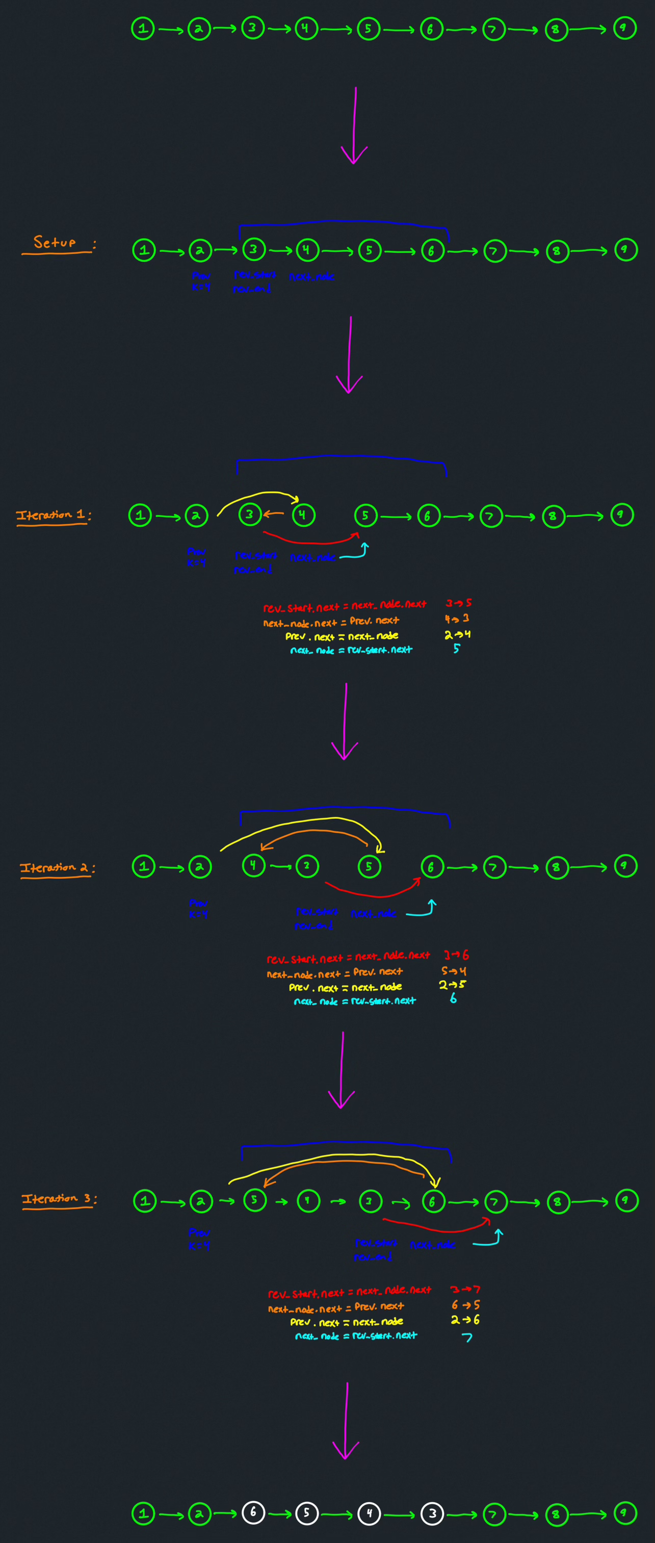
def reverse_k_nodes(prev, k):
if not prev.next or k < 2: # not possible to reverse at least 2 nodes (early return)
return prev.next
rev_start = prev.next # start node of segment to reverse
next_node = rev_start.next # next node to be moved in front of start node
rev_end = rev_start # start node of reversed segment will eventually be its last node, which we return
count = 1
while count <= k - 1 and next_node: # k - 1 iterations to move k - 1 nodes before start node (in reverse order)
rev_start.next = next_node.next # point start node to next node to be processed
next_node.next = prev.next # point node being moved before start node to current beginning node of reversed segment
prev.next = next_node # ensure node before reversed segment points to new start node of reversed segment (i.e., the node being moved)
next_node = rev_start.next # prepare for next node to be processed
count += 1 # keep track of iteration count to ensure proper termination
return rev_end # return last node of newly reversed segment
Examples
LC 92. Reverse Linked List II (✓) ★★
Reverse a linked list from position m to n. Do it in one-pass.
Note: 1 <= m <= n <= length of list
class Solution:
def reverseBetween(self, head: Optional[ListNode], left: int, right: int) -> Optional[ListNode]:
def reverse_k_nodes(prev, k):
if not prev.next or k < 2:
return prev.next
rev_start = prev.next
next_node = rev_start.next
rev_end = rev_start
count = 1
while count <= k - 1 and next_node:
rev_start.next = next_node.next
next_node.next = prev.next
prev.next = next_node
next_node = rev_start.next
count +=1
return rev_end
sentinel = ListNode(-1)
sentinel.next = head
prev = sentinel
for _ in range(left - 1):
prev = prev.next
reverse_k_nodes(prev, right - left + 1)
return sentinel.next
Time: . The entire list is processed in a linear fashion.
Space: . Additional memory is not consumed as the input size grows.
The template for reversing k nodes in-place was born out of the efforts to find a nice solution for this problem. The main potential "gotcha" is when left = 1, where the prev we need to feed into reverse_k_nodes needs to be a sentinel node.
LC 2074. Reverse Nodes in Even Length Groups (✓) ★★★
You are given the head of a linked list.
The nodes in the linked list are sequentially assigned to non-empty groups whose lengths form the sequence of the natural numbers (1, 2, 3, 4, ...). The length of a group is the number of nodes assigned to it. In other words,
- The
1stnode is assigned to the first group. - The
2ndand the 3rd nodes are assigned to the second group. - The
4th,5th, and6thnodes are assigned to the third group, and so on. Note that the length of the last group may be less than or equal to1 + the length of the second to last group.
Reverse the nodes in each group with an even length, and return the head of the modified linked list.
class Solution:
def reverseEvenLengthGroups(self, head: Optional[ListNode]) -> Optional[ListNode]:
def reverse_k_nodes(prev, k):
if not prev.next or k < 2:
return prev.next
rev_start = prev.next
next_node = rev_start.next
rev_end = rev_start
count = 1
while count <= k - 1 and next_node:
rev_start.next = next_node.next
next_node.next = prev.next
prev.next = next_node
next_node = rev_start.next
count += 1
return rev_end
if not head or not head.next:
return head
sentinel = ListNode(-1)
sentinel.next = head
connector = sentinel
curr = head
grp_size = count = 1
while curr:
if grp_size == count or not curr.next:
if count % 2 == 0:
curr = reverse_k_nodes(connector, count)
connector = curr
count = 0
grp_size += 1
count += 1
curr = curr.next
return sentinel.next
This is such an excellent problem. The solution above, originally inspired by this one, is brilliant in how it fulfills the problem's requirements and deftly utilizes reversing a specified number of nodes in place.
How does the solution logic work apart from reverse_k_nodes? First, recall what reverse_k_nodes does apart from reversing k nodes in-place: it returns the last node of the reversed segment. With this in mind, there are a few key points to highlight to illustrate how and why the solution above works:
-
We will maintain a
connectornode that allows us to keep all groups of the list connected. This node will always directly precede the beginning of a group. -
It's easy to get lost in keeping track of the odd or even groups, especially since the last group has to be treated differently than all the rest. A clever way of treating everything in a uniform fashion is to keep track of what the current group's full size would be,
grp_sizeas well as the current node count,count, as we move our way through the list. -
How do we move from one group to another effectively? We do so by determining whether or not the current node count equals the full size of the current group (i.e.,
grp_size == count) or if there aren't any nodes left to process, in which case we are done iterating and need to process the last group (i.e.,not curr.next).In both cases mentioned above, if the number of nodes in the group is even, then we need to reverse all these nodes in the group, and then continue on. Since
reverse_k_nodesreturns the last node of the newly reversed segment, we can setcurrequal to this function's return value. What remains is to setconnect = currbefore moving to the next group. We also add1to the next group's size,grp_size += 1, and we resetcount = 0because we add1tocountafter the if block no matter what happens.
LC 25. Reverse Nodes in k-Group (✓)
k is a positive integer and is less than or equal to the length of the linked list. If the number of nodes is not a multiple of k then left-out nodes, in the end, should remain as it is.
Follow up:
- Could you solve the problem in extra memory space?
- You may not alter the values in the list's nodes, only nodes itself may be changed.
class Solution:
def reverseKGroup(self, head: Optional[ListNode], k: int) -> Optional[ListNode]:
def reverse_k_nodes(prev, k):
if not prev.next or k < 2:
return prev.next
rev_start = prev.next
next_node = rev_start.next
rev_end = rev_start
count = 1
while count <= k - 1 and next_node:
rev_start.next = next_node.next
next_node.next = prev.next
prev.next = next_node
next_node = rev_start.next
count += 1
return rev_end
if not head or not head.next:
return head
sentinel = ListNode(-1)
sentinel.next = head
connector = sentinel
curr = head
grp_size = k
count = 1
while curr:
if count == k:
curr = reverse_k_nodes(connector, count)
count = 0
connector = curr
count += 1
curr = curr.next
return sentinel.next
This problem is very similar to LC 2074. Reverse Nodes in Even Length Groups. In fact, this problem is actually easier than that problem!
Swap two nodes
Remarks
TLDR: Don't overthink what seems like the tricky edge case of swapping adjacent nodes. The lengthy initial condition simply ensures we don't try to swap nodes that don't exist or identical nodes in memory.
Let left and right be the nodes we want to swap. We will need the nodes prior to left and right to facilitate the node swapping. Let these nodes be prev_left and prev_right, respectively. Most node swaps will look something like the following:
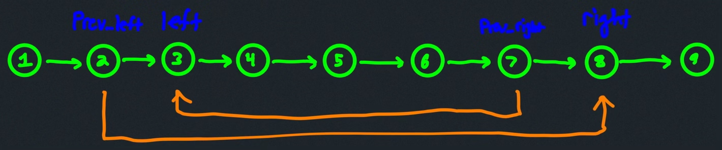
That is, as the figure suggests, we will first make the assignment prev_left.next = right and then prev_right.next = left. Now we need right.next to point to what left.next was pointing to, and we need left.next to point to what right.next was pointing to. We can do this without a temporary variable in Python: right.next, left.next = left.next, right.next.
Great! But what about the seemingly tricky case when nodes are adjacent? The really cool thing is that the template handles this case seamlessly. For the example figure above, consider what would happen if we tried swapping nodes 4 and 5:
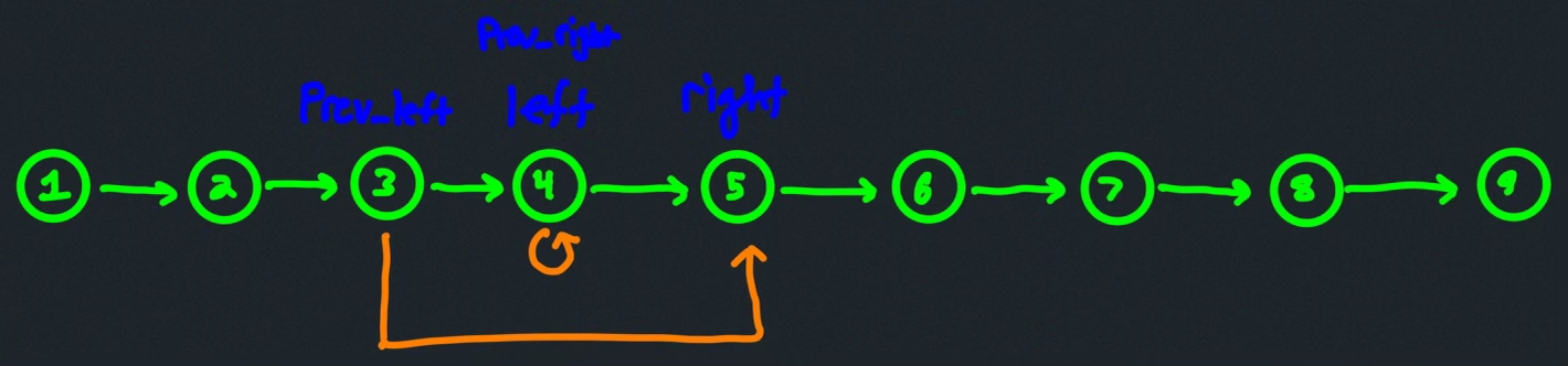
The assignment prev_left.next = right behaves as expected, but the assignment prev_right.next = left seems like it could cause some issues because we have effectively created a self-cycle. But the beautiful thing is how this is exploited to restore the list in the next set of assignments:
right.next, left.next = left.next, right.next
When nodes left and right are adjacent, we want right.next to point to left. The assignment right.next = left.next accomplishes exactly this because the self-cycle means left.next actually points to itself (i.e., left). The subsequent assignment left.next = right.next effectively removes the self-cycle and restores the list, resulting in the adjacent left and right nodes being swapped, as desired.
def swap_nodes(prev_left, prev_right):
if ( # determine whether or not it makes sense to try to swap nodes (return early if not)
not prev_left or # anchor node before left node to be swapped
not prev_right or # anchor node before right node to be swapped
not prev_left.next or # left node to be swapped
not prev_right.next or # right node to be swapped
prev_left.next == prev_right.next # test if nodes are identical in memory
):
return
left = prev_left.next # actual left node to be swapped
right = prev_right.next # actual right node to be swapped
prev_left.next, prev_right.next = right, left # adjust anchor pointers
right.next, left.next = left.next, right.next # adjust swapped node pointers
Examples
LC 24. Swap Nodes in Pairs (✓)
Given a linked list, swap every two adjacent nodes and return its head.
class Solution:
def swapPairs(self, head: Optional[ListNode]) -> Optional[ListNode]:
def swap_nodes(prev_left, prev_right):
if not prev_left or not prev_right \
or not prev_left.next or not prev_right.next \
or prev_left.next == prev_right.next:
return
left = prev_left.next
right = prev_right.next
prev_left.next, prev_right.next = right, left
right.next, left.next = left.next, right.next
if not head or not head.next:
return head
sentinel = ListNode(-1)
sentinel.next = head
prev_left = sentinel
prev_right = sentinel.next
while prev_left and prev_right:
swap_nodes(prev_left, prev_right)
prev_left = prev_right
prev_right = prev_right.next
return sentinel.next
The while loop condition conveys that we are only ever interested in trying to swap two nodes if both of their predecessors exist. Since this problem involves swapping pairs of nodes (i.e., the nodes are adjacent), the prev_left condition in the while loop is actually unnecessary (prev_right can only be true if prev_left is also true).
The main potential "gotcha" occurs after the swapping of the nodes. Note that prev_left and prev_right are never reassigned during the node swapping but their next attributes are. This means we need to be somewhat careful when making reassignments. As always, a drawing of a simple example can be immensely helpful:

Now the solution above basically suggests itself.
LC 1721. Swapping Nodes in a Linked List (✓)
You are given the head of a linked list, and an integer k.
Return the head of the linked list after swapping the values of the kth node from the beginning and the kth node from the end (the list is 1-indexed).
class Solution:
def swapNodes(self, head: Optional[ListNode], k: int) -> Optional[ListNode]:
def swap_nodes(prev_left, prev_right):
if not prev_left or not prev_right \
or not prev_left.next or not prev_right.next \
or prev_left.next == prev_right.next:
return
left = prev_left.next
right = prev_right.next
prev_left.next, prev_right.next = right, left
right.next, left.next = left.next, right.next
sentinel = ListNode(-1)
sentinel.next = head
prev_left = prev_right = sentinel
null_checker = head
for _ in range(k - 1):
prev_left = prev_left.next
null_checker = null_checker.next
while null_checker.next:
prev_right = prev_right.next
null_checker = null_checker.next
swap_nodes(prev_left, prev_right)
return sentinel.next
The motivation for the "swap two nodes" template really comes from this problem. Coming up with the template is the harder part — now all we have to do is work on identifying which nodes precede the left and right nodes.
General
Problems
LC 203. Remove Linked List Elements (✓)
Given the head of a linked list and an integer val, remove all the nodes of the linked list that has Node.val == val, and return the new head.
class Solution:
def removeElements(self, head: Optional[ListNode], val: int) -> Optional[ListNode]:
sentinel = ListNode(-1)
sentinel.next = head
prev = sentinel
curr = prev.next
while curr:
if curr.val == val:
prev.next = prev.next.next
else:
prev = curr
curr = curr.next
return sentinel.next
The key idea is that we only ever actually move prev when a non-val number is encountered; otherwise, we simply skip or "delete" nodes via prev.next = prev.next.next while constantly moving forward through the list with curr = curr.next.
LC 1290. Convert Binary Number in a Linked List to Integer (✓)
Given head which is a reference node to a singly-linked list. The value of each node in the linked list is either 0 or 1. The linked list holds the binary representation of a number.
Return the decimal value of the number in the linked list.
class Solution:
def getDecimalValue(self, head: ListNode) -> int:
curr = head
ans = curr.val
while curr.next:
ans = ans * 2 + curr.next.val
curr = curr.next
return ans
The idea behind the clever solution above is easier to understand if we first consider a simple base-10 number by itself: 4836. What this means in a base-10 system is the following (the powers of 10 indicate positional significance of the different numerals): .
How does this help with this problem? Well, consider how the number 4836 could be obtained if we encountered the digits one at a time, left to right:
ans = 4
= 4 * 10 + 8 -> (48)
= 48 * 10 + 3 -> (483)
= 483 * 10 + 6 -> (4836)
= 4836
The same thing is happening in this problem with respect to another base, namely base 2. For example, consider how the process above would look for the following number (in base 2): 101101:
ans = 1
= 1 * 2 + 0 -> (2)
= 2 * 2 + 1 -> (5)
= 5 * 2 + 1 -> (11)
= 11 * 2 + 0 -> (22)
= 22 * 2 + 1 -> (45)
= 45
The solution above is elegant in exploiting this instead of doing something else unnecessary like reversing the list and then updating the answer as we go along (which might be the first solution idea):
class Solution:
def getDecimalValue(self, head: ListNode) -> int:
def reverse(node):
prev = None
curr = node
while curr:
next_node = curr.next
curr.next = prev
prev = curr
curr = next_node
return prev
curr = reverse(head)
ans = 0
pos = 0
while curr:
if curr.val == 1:
ans += 2 ** pos
curr = curr.next
pos += 1
return ans
LC 328. Odd Even Linked List (✓) ★★
Given the head of a singly linked list, group all the nodes with odd indices together followed by the nodes with even indices, and return the reordered list.
The first node is considered odd, and the second node is even, and so on.
Note that the relative order inside both the even and odd groups should remain as it was in the input.
class Solution:
def oddEvenList(self, head: Optional[ListNode]) -> Optional[ListNode]:
if not head or not head.next:
return head
odd = head
even = odd.next
even_list_head = even
while even and even.next:
odd.next = odd.next.next
even.next = even.next.next
odd = odd.next
even = even.next
odd.next = even_list_head
return head
This is a great problem, but it is easy to overthink it and get bogged down in how the "node swapping" will work; in fact, that's the first problem! There is no node swapping! It's easy to fall into the trap of thinking we'll need to swap nodes to make the solution here work. A much more straightforward solution exists (i.e., the one above) if we can step outside the normal way of thinking here: what if we basically just created two lists, the odd list of the odd-index nodes and the even list of the even-index nodes? Then we could attach the even list to the odd list and call it a day.
And the idea above is completely possible. It just takes a little bit of imagination to execute it effectively. Specifically, what we have to be okay with (even though it may not seem okay in the moment) is effectively skipping or "deleting" the even-index nodes while dynamically creating the odd list and the same for the odd-index nodes while dynamically creating the even list.
Note that the while loop condition above is critical for the solution approach described above to work. We only care to continue building our lists so long as there are nodes that need to be repositioned; that is, we should only continue building our lists while an odd-indexed node appears after an even-indexed node. So long as this is true, we have work to do.
Matrices
Calculate value in a 2D matrix given its index
Remarks
index // n: This performs integer division ofindexbyn, where the result is the number of timesnfully goes intoindex. Why does this give us the row number? Because, for every row, there arenelements; hence, after everynelements, we move on to the next row.index % n: This finds the remainder whenindexis divided byn, where this remainder corresponds to the column index because it tells us how many places into the current row we are.
def index_to_value(matrix, index):
n = len(matrix[0])
row_pos = index // n
col_pos = index % n
return matrix[row_pos][col_pos]
Examples
LC 74. Search a 2D Matrix
Write an efficient algorithm that searches for a value in an m x n matrix. This matrix has the following properties:
- Integers in each row are sorted from left to right.
- The first integer of each row is greater than the last integer of the previous row.
class Solution:
def searchMatrix(self, matrix: List[List[int]], target: int) -> bool:
def index_to_mat_val(index):
row = index // n
col = index % n
return matrix[row][col]
m = len(matrix)
n = len(matrix[0])
left = 0
right = m * n - 1
while left <= right:
mid = left + (right - left) // 2
val = index_to_mat_val(mid)
if target < val:
right = mid - 1
elif target > val:
left = mid + 1
else:
return True
return False
Sliding window
Restarting window
Remarks
"Restarting" windows are for problems where we're tasked with not only optimizing a certain property of a 1-dimensional input (oftentimes maximizing the length of a subarray or substring) but also where we may encounter elements which cause the entire window to become invalid, thus forcing us to start again from an empty window (i.e., left == right).
Mechanically, how restarting windows work is that the right pointer advances one by one, as usual, expanding the window, but the left pointer remains fixed until an element is encountered that effectively invalidates the entire window. When this happens, we need to start again with an empty window, which means moving the left pointer to wherever the right pointer resides (recall that left == right means we have an empty window), thus effectively "resetting" the window.
Generally speaking, because the left pointer stays fixed until the window restarts, we don't even need the left pointer: we simply update the window data structures as we advance the right pointer and reset the data structures when the window restarts.
Note that we most often initialize/restart the window to be empty, but sometimes it is more convenient to always have a single element within the window. We initialize the window data structures and the result (the best window found so far) accordingly.
def fn(arr):
structs = ... # window data structures initialized for the starting window
ans = ... # value of the starting window (example: 0)
for right in range(1, len(arr) + 1): # the '1' depends on the starting window size
if WINDOW_IS_INVALID: # adding arr[right - 1] invalidates the window somehow
structs = ... # RESET data structures for maintaining the window
else:
structs += ... # UPDATE data structures to reflect addition of arr[right - 1] to the window
ans = max(ans, ...) # update ans if the current window is better
return ans
Examples
LC 485. Max Consecutive Ones (✠)
Given a binary array nums, return the maximum number of consecutive 1's in the array.
class Solution:
def findMaxConsecutiveOnes(self, nums: List[int]) -> int:
curr = ans = 0
for right in range(1, len(nums) + 1):
if nums[right - 1] != 1:
curr = 0
else:
curr += 1
ans = max(ans, curr)
return ans
Time: . Each element in nums is processed in time.
Space: . The memory consumed does not increase in proportion to the size of the input.
The solution above is nice and neat, but it's worth discussing this problem more as a quintessential example of the "restarting window" template in action. The window property/constraint in this problem is to "contain only 1's", and the goal is to maximize the length of whatever subarrays we can find that satisfy this constraint.
Note that any window that contains a 0 is invalid; hence, encountering a 0 causes whatever window we're maintaining to restart. The sequence of sliding windows would look like the image below, where each row shows one window in red — a single vertical red line denotes an empty window where the two pointers are at the same index (i.e., left == right). We start with an empty window (i.e., left = 0, right = 0, left == right) and stop when right == len(nums), resulting in a final answer of 3 for the example below:
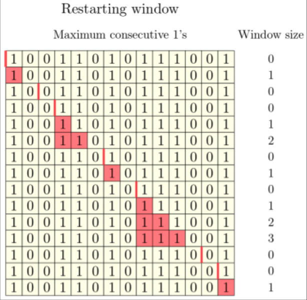
This process can be explicitly coded in the following manner:
class Solution:
def findMaxConsecutiveOnes(self, nums: List[int]) -> int:
left = 0 # `right = 0` is implied (start with an empty window)
ans = 0 # variable to keep track of the longest valid window encountered
for right in range(1, len(nums) + 1):
if nums[right - 1] != 1: # entire window invalidated (encountered element not 1)
left = right # restart the window to be empty
else:
ans = max(ans, right - left) # `right - left` gives the length of the current valid window
return ans
Since the left pointer is only being used for length calculations and it always skips ahead to right when we reset the window, most solutions that use a restarting window approach will not explicitly use a left pointer but instead maintain a data structure for each window and then just reset it when needed, as above:
class Solution:
def findMaxConsecutiveOnes(self, nums: List[int]) -> int:
curr = ans = 0 # curr denotes size of current valid window (ans the largest found)
for right in range(1, len(nums) + 1):
if nums[right - 1] != 1:
curr = 0 # restart size of current valid window to `0`
else:
curr += 1
ans = max(ans, curr)
return ans
LC 1446. Consecutive Characters (✠)
Given a string s, the power of the string is the maximum length of a non-empty substring that contains only one unique character.
Return the power of the string.
class Solution:
def maxPower(self, s: str) -> int:
curr_char = s[0]
curr = power = 1
for right in range(2, len(s) + 1):
if s[right - 1] != curr_char:
curr_char = s[right - 1]
curr = 1
else:
curr += 1
power = max(power, curr)
return power
Time: . We process all elements in nums and it takes time to process each element.
Space: . The memory consumed does not increase in proportion to the input size.
Note that this problem is an example of one where we always want the window to have a single element (the current character being considered).
LC 53. Maximum Subarray (✠)
Given an integer array nums, find the contiguous subarray (containing at least one number) which has the largest sum and return its sum.
class Solution:
def maxSubArray(self, nums: List[int]) -> int:
curr = ans = nums[0]
for right in range(2, len(nums) + 1):
if curr < 0:
curr = nums[right - 1]
else:
curr += nums[right - 1]
ans = max(ans, curr)
return ans
Time: . Every element of nums is processed, and it takes time to process each element.
Space: . The amount of memory consumed does not increase in proportion to the input size.
The code above is actually a reformulation of Kadane's algorithm, which uses some clever observations to process the entire array in linear time. The usual formulation of Kadane's algorithm is the following:
def max_subarray(numbers):
"""Find the largest sum of any contiguous subarray."""
best_sum = float('-inf')
current_sum = 0
for x in numbers:
current_sum = max(x, current_sum + x)
best_sum = max(best_sum, current_sum)
return best_sum
The highlighted line is the key to understanding why Kadane's algorithm works. If current_sum is negative (i.e., curr in our solution above), where current_sum denotes the current sum of the subarray/window we're currently considering/maintaining, then what could possibly be gained by extending the window to effectively decrease our running sum (i.e., if current_sum is negative, then x must be greater than current_sum + x)? It would be better if we simply restarted our window to contain only the number x.
The logic outlined above is easier to see in the usual formulation of Kadane's algorithm, but it doesn't change the fact that this is essentially a "restarting window" with a very clever observation to make it work. It's also worth noting that ans = max(ans, curr) occurs after the if/else block because the single element window upon restarting the window may sometimes be optimal.
Fixed window size
Remarks
TBD
Building the initial window within the main loop instead of outside the main loop
It is possible to build the initial k-size window within the main loop instead of as the result of a separate for loop. But just because we can do this doesn't mean we should. The result oftentimes looks unnatural, as in the solutions to the following two problems.
Problem: Max sum of subarray of size k
def find_best_subarray(nums, k):
curr = 0
ans = float('-inf')
for right in range(1, len(nums) + 1):
if right >= k + 1:
ans = max(curr, ans)
curr -= nums[right - k - 1]
curr += nums[right - 1]
ans = max(ans, curr)
return ans
nums = [3,-1,4,12,-8,5,6]
k = 4
print(find_best_subarray(nums, k)) # 18
def find_best_subarray(nums, k):
curr = 0
for right in range(1, k + 1):
curr += nums[right - 1]
ans = curr
for right in range(k + 1, len(nums) + 1):
curr += nums[right - 1]
curr -= nums[right - 1 - k]
ans = max(ans, curr)
return ans
nums = [3,-1,4,12,-8,5,6]
k = 4
print(find_best_subarray(nums, k)) # 18
Both approaches work, but the first approach is arguably less natural.
Problem: LC 643. Maximum Average Subarray I
class Solution:
def findMaxAverage(self, nums: List[int], k: int) -> float:
curr = 0
ans = float('-inf')
for right in range(1, len(nums) + 1):
if right >= k + 1:
ans = max(ans, curr / k)
curr -= nums[right - 1 - k]
curr += nums[right - 1]
ans = max(ans, curr / k)
return ans
class Solution:
def findMaxAverage(self, nums: List[int], k: int) -> float:
left = curr = 0
for right in range(1, k + 1):
curr += nums[right - 1]
ans = curr / k
for right in range(k + 1, len(nums) + 1):
curr += nums[right - 1]
curr -= nums[right - 1 - k]
ans = max(ans, curr / k)
return ans
Again, both approaches technically work, but the first approach seems to be less natural.
def fn(arr, k):
structs = ... # window data structures initialized for the starting window
for right in range(1, k + 1): # process k elements from indices 0 to k - 1, inclusive
structs += ... # update data structures to reflect addition of arr[right - 1] to window
ans = ... # value of the window of size k
for right in range(k + 1, len(arr) + 1): # process remaining elements in input
structs += ... # update data structures to reflect addition of arr[right - 1] to window
structs -= ... # update data structures to reflect removal of arr[right - 1] from window
ans = max(ans, ...) # update ans if the current window is better
return ans
Examples
Max sum of subarray of size k (✓)
def find_best_subarray(nums, k):
curr = 0
for right in range(1, k + 1):
curr += nums[right - 1]
ans = curr
for right in range(k + 1, len(nums) + 1):
curr += nums[right - 1]
curr -= nums[right - 1 - k]
ans = max(ans, curr)
return ans
The idea here is that we first build the sum of the first window of size k. Then we continue onward by adding and removing elements from the k-size window while keeping track of the current window sum and comparing that to the maximum, the final of which we return as the ultimate answer.
Time: . The i pointer will move a total of units where n == len(nums).
Space: . No additional space is consumed in proportion to the input.
LC 643. Maximum Average Subarray I (✓)
You are given an integer array nums consisting of n elements, and an integer k.
Find a contiguous subarray whose length is equal to k that has the maximum average value and return this value. Any answer with a calculation error less than 10-5 will be accepted.
class Solution:
def findMaxAverage(self, nums: List[int], k: int) -> float:
left = curr = 0
for right in range(1, k + 1):
curr += nums[right - 1]
ans = curr / k
for right in range(k + 1, len(nums) + 1):
curr += nums[right - 1]
curr -= nums[right - 1 - k]
ans = max(ans, curr / k)
return ans
Time: . The entire nums array is processed, where n == len(nums).
Space: . No additional space is consumed in proportion to the input size.
Most 1s in subarray of size k (✠, 💎)
def maxOnes(nums, k):
curr = 0
for right in range(1, k + 1):
if nums[right - 1] == 1:
curr += 1
ans = curr
for right in range(k + 1, len(nums) + 1):
if nums[right - 1] == 1:
curr += 1
if nums[right - 1 - k] == 1:
curr -= 1
ans = max(ans, curr)
return ans
Time: . Each element of nums is processed and is done so in time.
Space: . Additional memory is not consumed as the input grows in size.
Since we want to increase the count when a 1 is encountered and enters the window and decrease the count when a 1 leaves the window, we can clean up the code above to be a bit more concise:
def maxOnes(nums, k):
curr = 0
for right in range(1, k + 1):
curr += nums[right - 1]
ans = curr
for right in range(k + 1, len(nums) + 1):
curr += nums[right - 1]
curr -= nums[right - 1 - k]
ans = max(ans, curr)
return ans
But this is mostly a consequence of the fact that we're increasing the count when we encounter a 1, which is exactly what we need to add (or remove) from the cumulative sum being maintained. If, instead, we wanted to keep track of the maximum number of 8's in a subarray of length 5, then the cleanup done above would not work, and we would need to revert back to something like the original solution at the beginning.
Ultimately, the window property or constraint for this problem is to "have length k", and what we're trying to optimize is the number of 1's in a k-length subarray. We start with a window of length k, where left = 0 is implied and right = k. This corresponds to building the k-length window within the following block:
for right in range(1, k + 1):
# ...
We process the rest of the fixed-length subarrays/windows in the following block (we stop when right == len(nums)):
for right in range(k + 1, len(nums) + 1):
# ...
Worth noting is how we don't actually need a left pointer: each time right is incremented, we implicitly increment left; that is, incrementing right corresponds to adding nums[right - 1] to our window, and implicitly incrementing left corresponds to removing nums[right - 1 - k] from our window. Why?
Once the initial window is built, we see that our subarray or window spans the interval [0, k), where left == 0 and right == k. In general, for a k-length window, if we have left = x, then we will have right = x + k, where the length of the window is given by right - left == (x + k) - x == k and can be represented in interval notation as [x, x + k).
What happens if our window shifts one unit to the right? We will still have [x, x + k), where right = x + k, but the previous window is now represented differently:
To maintain our window, we need to remove the value highlighted in red above, and we need to add the value highlighted in green. Since right = x + k, the value we need to add to our window is
nums[x + k - 1] == nums[(x + k) - 1] = nums[right - 1]
and the value we need to remove from our window is
nums[x - 1] = nums[(right - k) - 1] = nums[right - 1 - k]
where above we make use of the fact that x = right - k follows from the fact that right = x + k.
Ultimately, the sequence of sliding windows looks like the image below, where nums = [1,0,0,1,1,0,1,0,1,1,1,0,0,1] and k = 5:
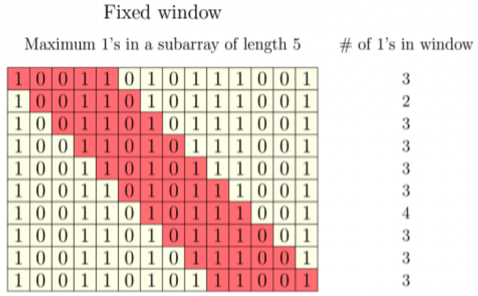
Each row shows a k-length window in red (k = 5 in this example). We stop when right = len(arr).
LC 1456. Maximum Number of Vowels in a Substring of Given Length (✓, ✠)
Given a string s and an integer k.
Return the maximum number of vowel letters in any substring of s with length k.
Vowel letters in English are (a, e, i, o, u).
class Solution:
def maxVowels(self, s: str, k: int) -> int:
vowels = { 'a', 'e', 'i', 'o', 'u' }
curr = 0
for right in range(1, k + 1):
if s[right - 1] in vowels:
curr += 1
ans = curr
for right in range(k + 1, len(s) + 1):
if s[right - 1] in vowels:
curr += 1
if s[right - 1 - k] in vowels:
curr -= 1
ans = max(ans, curr)
return ans
Time: . Each character in s is processed in time.
Space: . The set with the vowels is the only additionally allocated space, and it does not increase with an increased size in the input.
LC 567. Permutation in String (✓, ✠)
Given two strings s1 and s2, write a function to return true if s2 contains the permutation of s1. In other words, one of the first string's permutations is the substring of the second string.
class Solution:
def checkInclusion(self, s1: str, s2: str) -> bool:
if len(s1) > len(s2): # impossible for any permutation of s1 to be a substring of s2
return False
k = len(s1) # maintain fixed-width window of size k where k = len(s1)
surplus = defaultdict(int) # hash map to keep track of surplus values
for char in s1: # start with a deficit of excess occurrences
surplus[char] -= 1
for right in range(1, k + 1): # build the initial window of size k
surplus[s2[right - 1]] += 1 # adjust surplus values accordingly
mismatches = sum(abs(surplus[char]) for char in surplus) # calculate number of mismatches
if mismatches == 0: # if no mismatches found, then permutation already discovered
return True
for right in range(k + 1, len(s2) + 1):
if surplus[s2[right - 1]] < 0: # if there is a deficit of the character we're about to add to the window,
mismatches -= 1 # then decrease the number of mismatches by 1 (the number of mismatches
else: # will decrease by 1 once the number is actually added to the window)
mismatches += 1 # if no deficit, then we just created another mismatch by
# adding an unnecessary character to the window
surplus[s2[right - 1]] += 1 # actually add the character to the window
if surplus[s2[right - 1 - k]] > 0: # if there is a surplus of the character we're about to remove from the window,
mismatches -= 1 # then decrease the number of mismatches by 1 (the number of mismatches
else: # will decrease by 1 once the number is actually removed from the window)
mismatches += 1 # if there was no surplus, then removing the character from the window
# introduces a mismatch (increment mismatch total by 1)
surplus[s2[right - 1 - k]] -= 1 # actually remove the character from the window
if mismatches == 0: # if no mismatches are found after adding and removing from the k-length window,
return True # then the current window/substring of s2 must be a permutation of s1
return False # mismatches still exist (no permutation found)
Time: . The left and right pointers can iterate a total number of n times where n = len(s2).
Space: . The space is technically since the character set only has characters, meaning .
Why is a fixed-width sliding window appropriate here? Because no matter how we permute the characters of s1, the "block" of permuted characters must appear as a "block" (i.e., substring) in s2; hence, if we let k = len(s1), then the goal is to efficiently consider all k-length windows of s2 (i.e., all substrings of length k in s2).
How can we do this efficiently? The idea is to maintain a sort of ledger that maps each letter to the number of excess occurrences of that letter in the window relative to s1. Let surplus serve the role of this ledger (implemented as a hash map). For example,
- if
surplus['a'] = 3, then this means that the current window has3morea's than the number ofa's ins1. Conversely, - if
surplus['a'] = -3, then this means that the current window has3fewera's than the number ofa's ins1. Finally, - if
surplus['a'] = 0, then this means that the current window has the same number ofa's as the number ofa's ins1.
The window (i.e., substring of s2) is a permutation of s1 when all surplus values are 0.
To avoid summing all surplus values after each iteration, we instead keep track of the sum of the absolute value of all surplus values in the mismatches variable (the absolute value is used because we want to avoid situations where a positive surplus cancels out a negative surplus) — if that sum is 0, then we have found a permutation.
Each time we slide the window, we need to update both window data structures: the surplus ledger and the mismatches sum.
LC 438. Find All Anagrams in a String (✠)
Given two strings s and p, return an array of all the start indices of p's anagrams in s. You may return the answer in any order.
class Solution:
def findAnagrams(self, s: str, p: str) -> List[int]:
if len(p) > len(s): # impossible for any permutation of p to be a substring of s
return []
k = len(p) # maintain fixed-width window of size k where k = len(p)
surplus = defaultdict(int) # hash map to keep track of surplus values
for char in p: # start with a deficit of excess occurrences
surplus[char] -= 1
for right in range(1, k + 1): # build the initial window of size k
surplus[s[right - 1]] += 1 # adjust surplus values accordingly
mismatches = sum(abs(surplus[char]) for char in surplus) # calculate number of mismatches
anagrams = []
if mismatches == 0: # if no mismatches found, then permutation discovered starting at index 0
anagrams.append(0)
for right in range(k + 1, len(s) + 1):
if surplus[s[right - 1]] < 0: # if there is a deficit of the character we're about to add to the window,
mismatches -= 1 # then decrease the number of mismatches by 1 (the number of mismatches
else: # will decrease by 1 once the number is actually added to the window)
mismatches += 1 # if no deficit, then we just created another mismatch by
# adding an unnecessary character to the window
surplus[s[right - 1]] += 1 # actually add the character to the window
if surplus[s[right - 1 - k]] > 0: # if there is a surplus of the character we're about to remove from the window,
mismatches -= 1 # then decrease the number of mismatches by 1 (the number of mismatches
else: # will decrease by 1 once the number is actually removed from the window)
mismatches += 1 # if there was no surplus, then removing the character from the window
# introduces a mismatch (increment mismatch total by 1)
surplus[s[right - 1 - k]] -= 1 # actually remove the character from the window
if mismatches == 0: # if no mismatches are found after adding and removing from the k-length window,
anagrams.append(right - k) # then the current window/substring of s must be a permutation of p:
# [L, right) ... [L, right - 1] ... length: (right - 1) - (L) + 1 = k -> L = right - k
return anagrams # return all anagrams
Time: . This is almost the same as the following problem: LC 567. Permutation in String, but instead we aggregate permutations by collecting their starting indices instead of immediately returning true once one is found.
Space: . The anagrams output is not included in the overal space cost since it is the expected return value.
LC 2090. K Radius Subarray Averages (✓)
You are given a 0-indexed array nums of n integers, and an integer k.
The k-radius average for a subarray of nums centered at some index i with the radius k is the average of all elements in nums between the indices i - k and i + k (inclusive). If there are less than k elements before or after the index i, then the k-radius average is -1.
Build and return an array avgs of length n where avgs[i] is the k-radius average for the subarray centered at index i.
The average of x elements is the sum of the x elements divided by x, using integer division. The integer division truncates toward zero, which means losing its fractional part.
- For example, the average of four elements
2,3,1, and5is(2 + 3 + 1 + 5) / 4 = 11 / 4 = 2.75, which truncates to2.
class Solution:
def getAverages(self, nums: List[int], k: int) -> List[int]:
n = len(nums)
curr = 0
subarray_width = 2 * k + 1
res = []
# not possible to have any k-radius subarray averaged
if subarray_width > n:
return [-1] * n
# build fixed-width window of size subarray_width
for right in range(1, subarray_width + 1):
curr += nums[right - 1]
# k-radius subarray average not possible for first k values
for _ in range(k):
res.append(-1)
# main window logic
res.append(curr // subarray_width) # add first k-radius subarray average to the results list
for right in range(subarray_width + 1, len(nums) + 1):
curr += nums[right - 1]
curr -= nums[right - 1 - subarray_width]
res.append(curr // subarray_width)
# k-radius subarray average not possible for last k values
for _ in range(k):
res.append(-1)
return res
Time: . It takes time to process all elements and to add -1 when a k-radius subarray average is not possible Processing each element takes time.
Space: . A constant amount of space is used regardless of input size.
LC 3364. Minimum Positive Sum Subarray
You are given an integer array nums and two integers l and r. Your task is to find the minimum sum of a subarray whose size is between l and r (inclusive) and whose sum is greater than 0.
Return the minimum sum of such a subarray. If no such subarray exists, return -1.
A subarray is a contiguous non-empty sequence of elements within an array.
class Solution:
def minimumSumSubarray(self, nums: List[int], l: int, r: int) -> int:
n = len(nums)
# build prefix sum
prefix = [nums[0]]
for i in range(1, n):
prefix.append(prefix[-1] + nums[i])
ans = float('inf')
# process all subarrays of length l, l + 1, ... , r (inclusive)
for subarray_size in range(l, r + 1):
curr = prefix[subarray_size - 1] # calculate total sum of first `subarray_size` elements in `nums` in O(1) time
if curr > 0:
ans = min(ans, curr) # update the answer if the running sum is actually positive
for right in range(subarray_size + 1, n + 1): # use fixed-width sliding window of length `subarray_size` to process all elements
curr += nums[right - 1]
curr -= nums[right - 1 - subarray_size]
if curr > 0:
ans = min(ans, curr)
return ans if ans != float('inf') else -1
Time: .
Space: .
Using a prefix sum in the solution above makes it possible for us to avoid incurring a deeply nested call to compute sums, which would leave us with the brute-force algorithm that takes time:
class Solution:
def minimumSumSubarray(self, nums: List[int], l: int, r: int) -> int:
res = float('inf')
for i in range(len(nums)): # O(n)
for j in range(i, len(nums)): # O(n)
if l <= j - i + 1 <= r:
subarray_sum = sum(nums[i:j+1]) # O(n)
if subarray_sum > 0:
res = min(res, subarray_sum)
return res if res != float('inf') else - 1 # T: O(n^3); S: O(1)
The idea is to pre-process nums to build a prefix sum so that we can effectively use a fixed-width sliding window.
Variable window size (maximum)
Remarks
The general algorithm behind the sliding window pattern (variable width) is as follows:
- Define window boundaries: Define pointers
leftandrightthat bound the left- and right-hand sides of the current window, respectively, where both pointers usually start at0. - Add elements to window by moving right pointer: Iterate over the source array with the
rightbound to "add" elements to the window. - Remove elements from window by checking constraint and moving left pointer: Whenever the constraint is broken, "remove" elements from the window by incrementing the
leftbound until the constraint is satisfied again.
Note the usage of the non-strict inequality left <= right in the while loop — this makes sense for problems where a single-element window is valid; however, the inequality should be strict (i.e., left < right) for problems where a single-element window does not make sense.
Note the possibility of using ans += right - left + 1 instead of ans = max(ans, right - left + 1) when considering problems that require us to count the number of valid subarrays satisfying some constraint (e.g., LC 713. Subarray Product Less Than K). This approach is only relevant when all other subarrays of a valid subarray must also be valid; that is, for example, in the case of LC 713, all array values are positive so any subarray of a valid subarray must necessarily also be valid (because the product of all of its elements will be smaller). Essentially, there has to be some kind of "monotonicity" to the problem for this approach to work. Hence, this approach for counting the number of subarrays will not come up often, but it is definitely worth being aware of because it makes quick work of what might otherwise be a difficult problem.
Concretely: If the subarray/window [left, right] is valid and all of its subarrays are also valid, then how many valid subarrays are there that end at index right? There are right - left + 1 in total: [left, right], [left + 1, right], [left + 2, right], and so on until we reach [right, right] (i.e., the single-element window at right). Hence, the number of valid windows/subarrays ending at index right is equal to the size of the window, which we know is right - left + 1.
This clever "math trick" takes advantage of the sliding nature of the algorithm, where we always determine the number of valid subarrays ending at each index — this makes it easy to avoid overcounting and simplifies the determination process a great deal.
def fn(arr):
structs = ... # window data structures initialized for the starting window
ans = ... # value of the starting window (example: 0)
left = 0 # initialize left = 0 (explicit) and right = 0 (implied)
for right in range(1, len(arr) + 1):
structs = ... # update data structures to reflect addition of arr[right - 1] to window
while left < right and WINDOW_IS_INVALID: # adding arr[right - 1] invalidates the window somehow
structs = ... # update data structures to reflect removal of arr[right - 1] from window
left += 1 # shrink window until it either becomes or empty (left == right) or is valid again
ans = max(ans, right - left) # length of "valid" window
# ans += right - left # number of "valid" subarrays ending at 'right - 1' (when counting)
return ans
Examples
Longest subarray of positive integer array with sum not greater than k (✓)
def find_length(nums, k):
left = curr = ans = 0
for right in range(1, len(nums) + 1):
curr += nums[right - 1]
while left < right and curr > k:
curr -= nums[left]
left += 1
ans = max(ans, right - left)
return ans
Time: . The for loop can iterate a maximum number of times, where n = len(nums). The same is true for the while loop. Basically right is progressed units while left is progressed a maximum of units, meaning our overall time complexity is .
Space: . The space required does not scale with the input here, which means the space required is constant.
Longest substring of 1's given binary string and one possible 0 flip (✓)
def find_length(s):
left = curr = ans = 0
for right in range(1, len(s)):
if s[right - 1] == '0':
curr += 1
while left < right and curr > 1:
if s[left] == '0':
curr -= 1
left += 1
ans = max(ans, right - left)
return ans
Above, curr denotes the current number of zeroes in the window.
Time: . The right pointer moves units, where n = len(s), and left moves a maximum total of units, meaning the overall time complexity is .
Space: . The space used is constant proportional to the input.
LC 713. Subarray Product Less Than K (✓) ★
Your are given an array of positive integers nums.
Count and print the number of (contiguous) subarrays where the product of all the elements in the subarray is less than k.
class Solution:
def numSubarrayProductLessThanK(self, nums: List[int], k: int) -> int:
left = ans = 0
curr = 1
for right in range(1, len(nums) + 1):
curr *= nums[right - 1]
while left < right and curr >= k:
curr //= nums[left]
left += 1
ans += (right - left)
return ans
For a valid sliding window [left, right) that satisfies the condition and constraints, note that adding right - left to ans effectively adds the total number of subarrays in the range [left, right) that end at right - 1, inclusive.
This is a nifty trick we can use when the subarrays in question exhibit some sort of "monotonic" property; in this case, the product for positive integers uniformly increases as we add more positive integers to multiply (i.e., as the window becomes larger).
Time: . The right pointer moves a maximum of units, where n = len(nums), and left moves a maximum of units as well, meaning our overall time complexity is .
Space: . The space used does not grow in proportion to the size of the input. It is constant.
LC 1004. Max Consecutive Ones III (✓, ✠, 💎)
Given a binary array nums and an integer k, return the maximum number of consecutive 1's in the array if you can flip at most k 0's.
class Solution:
def longestOnes(self, nums: List[int], k: int) -> int:
left = curr = ans = 0
for right in range(1, len(nums) + 1):
if nums[right - 1] == 0:
curr += 1
while left < right and curr > k:
if nums[left] == 0:
curr -= 1
left += 1
ans = max(ans, right - left)
return ans
Time: . Each element in nums is processed in time.
Space: . Additional memory is not consumed in proportion to an increase in the input size.
Since we're interested in finding the longest subarray with some property, our goal is to maximize the window size as much as possible until we're forced to shrink it. Specifically, if we can grow the window by adding nums[right - 1] to it without making the window invalid, then we do so; otherwise, we shrink the window by removing nums[left] from it.
Maximum windows are like restarting windows in that they are intended for problems where we are trying to find a subarray/window that is as large as possible. The main difference is that, for maximum windows, we don't throw away the entire window once it becomes invalid; instead, we increment the left pointer one by one until we can expand the window again (i.e., until the window is either empty or becomes valid again).
For this problem specifically, it can help to rephrase the problem from
Given a binary array
numsand an integerk, return the maximum number of consecutive1's in the array if you can flip at mostk0's.
to
Given a binary array
numsand an integerk, return the length of the longest subarray containing at mostk0's.
The sequence of sliding windows then looks like the image below:
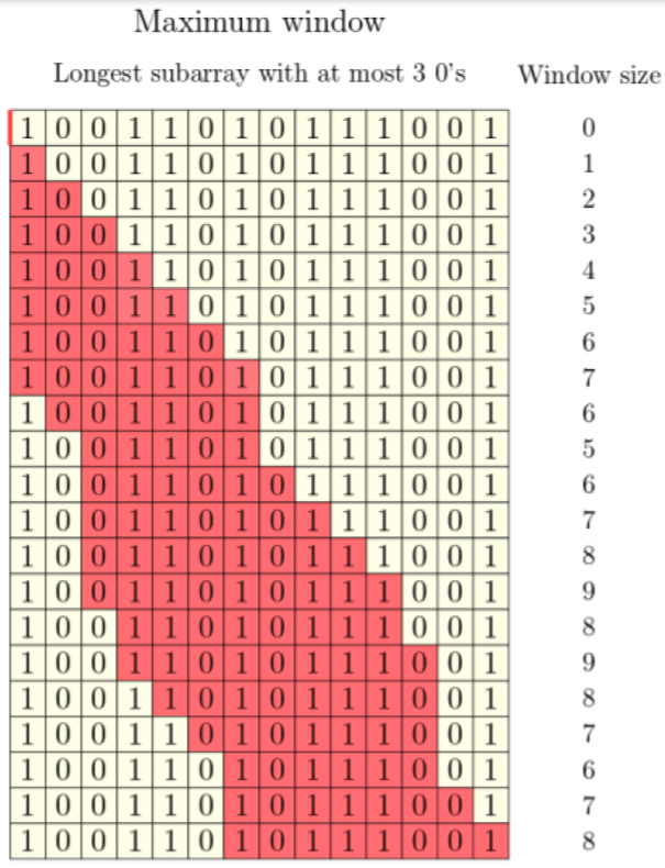
Each row shows one window in red, where we start with an empty window (i.e., left = 0 and right = 0). And we stop when right == len(nums). The final answer is 9.
LC 3. Longest Substring Without Repeating Characters (✓, ✠) ★★
Given a string s, find the length of the longest substring without repeating characters.
class Solution:
def lengthOfLongestSubstring(self, s: str) -> int:
left = ans = 0
freqs = defaultdict(int)
for right in range(1, len(s) + 1):
freqs[s[right - 1]] += 1
while left < right and freqs[s[right - 1]] > 1:
freqs[s[left]] -= 1
left += 1
ans = max(ans, right - left)
return ans
Time: . The left and right pointers both travel a maximum of units, where n == len(s).
Space: . A restricted character set is allowed, which means the hash map used for lookups cannot grow beyond a certain size, but we could say , where k allowed for more flexibility in characters.
The nature of this problem allows us to make a small optimization: as soon as we encounter a character that is a duplicate, instead of incrementing left one character at a time until that character's previous occurrence is encountered and skipped over, we use our hash map to track character indexes (not frequencies) and simply jump the left pointer just past the last index of the previously encountered duplicate character:
class Solution:
def lengthOfLongestSubstring(self, s: str) -> int:
left = ans = 0
lookup = dict()
for right in range(1, len(s) + 1):
if s[right - 1] in lookup and lookup[s[right - 1]] >= left:
left = lookup[s[right - 1]] + 1
lookup[s[right - 1]] = right - 1
ans = max(ans, right - left)
return ans
The hardest part about the solution above is the change in thinking needed to implement the variable width sliding window effectively. There's no while loop and the conventional "sliding" isn't so much sliding as it is "jumping". Additionally, the condition and lookup[char] >= left is critical for the sliding window — it ensures the character is not just in the hash map but that its last occurrence is within the current window. Our solution would fail without this conditional check.
For example, consider s = "abba". When we encounter the last "a", the first "a" is in the hash map, but it is not in the current window. Mistakenly treating it like it's part of the current window means moving the left pointer just past this occurrence and mistakenly getting a right - left length of 3, which is not correct.
LC 424. Longest Repeating Character Replacement (✠)
Given a string s that consists of only uppercase English letters, you can perform at most k operations on that string.
In one operation, you can choose any character of the string and change it to any other uppercase English character.
Find the length of the longest sub-string containing all repeating letters you can get after performing the above operations.
Note: Both the string's length and k will not exceed 104.
class Solution:
def characterReplacement(self, s: str, k: int) -> int:
left = curr_max = ans = 0
freqs = defaultdict(int)
for right in range(1, len(s) + 1):
freqs[s[right - 1]] += 1
curr_max = max(curr_max, freqs[s[right - 1]])
while left < right and right - left - curr_max > k:
freqs[s[left]] -= 1
curr_max = max(curr_max, freqs[s[left]])
left += 1
ans = max(ans, right - left)
return ans
Time: . The left and right pointers make a maximum of n iterations each, where n = len(s).
Space: . The frequency of each character is tracked which means the size is .
The key realization is to precisely define the window property/constraint that must be maintained: the window contains at most k characters which are not the most frequently occurring one. Hence, we keep a frequency count, freqs, of each character in the window, and we maintain a counter, curr_max, that maintains the current maximum frequency for any character in the window.
The idea is that the window, which may be represented by the interval [left, right), has length right - left, where the character that occurs most frequently occurs a total of curr_max times. Consequently, we can change up to k of the remaining (right - left) - curr_max characters to be the character that occurs most frequently so that the entire window is made up of the same character. But once (right - left) - curr_max exceeds k, then our window becomes invalid, and we must shrink it in order to make every character in the window the same character.
Examples (old way)
LC 209. Minimum Size Subarray Sum (✓)
Given an array of positive integers nums and a positive integer target, return the minimal length of a contiguous subarray [numsl, numsl+1, ..., numsr-1, numsr] of which the sum is greater than or equal to target. If there is no such subarray, return 0 instead.
class Solution:
def minSubArrayLen(self, target: int, nums: List[int]) -> int:
MAX_NUMS_LENGTH = 10 ** 5 + 1
left = 0
curr = 0
ans = MAX_NUMS_LENGTH
for right in range(len(nums)):
curr += nums[right]
while left <= right and curr >= target:
ans = min(ans, right - left + 1)
curr -= nums[left]
left += 1
return 0 if ans == MAX_NUMS_LENGTH else ans
Sometimes the standard template needs to be modified slightly. This problem is clearly asking to be solved via sliding window, but the most natural way of solving the problem does not conform completely to the template. That's okay. Specifically, we want the condition of the window to be met before we remove any elements and/or update the answer.
LC 1208. Get Equal Substrings Within Budget (✓)
You are given two strings s and t of the same length. You want to change s to t. Changing the ith character of s to ith character of t costs |s[i] - t[i]| that is, the absolute difference between the ASCII values of the characters.
You are also given an integer maxCost.
Return the maximum length of a substring of s that can be changed to be the same as the corresponding substring of t with a cost less than or equal to maxCost.
If there is no substring from s that can be changed to its corresponding substring from t, return 0.
class Solution:
def equalSubstring(self, s: str, t: str, maxCost: int) -> int:
def char_diff(char1, char2):
return abs(ord(char1) - ord(char2))
left = curr = ans = 0
for right in range(len(t)):
curr += char_diff(t[right], s[right])
while left <= right and curr > maxCost:
curr -= char_diff(t[left], s[left])
left += 1
ans = max(ans, right - left + 1)
return ans
The main idea here is that s is purely for reference while the sliding window operates by traversing t.
LC 3090. Maximum Length Substring With Two Occurrences★★
Given a string s, return the maximum length of a substring such that it contains at most two occurrences of each character.
class Solution:
def maximumLengthSubstring(self, s: str) -> int:
lookup = defaultdict(int)
left = ans = 0
for right in range(len(s)):
curr_char = s[right]
lookup[curr_char] += 1
while left <= right and lookup[curr_char] > 2:
prev_char = s[left]
lookup[prev_char] -= 1
left += 1
ans = max(ans, right - left + 1)
return ans
The idea is effectively to use a hash map to track the frequency of characters as we encounter them — as soon as a character occurs more than 2 times (the right boundary), move the left boundry until a valid window is attained (subtracting out the character frequencies from the hash map along the way).
Note how easy it is to extend this solution to a number k >= 2:
class Solution:
def maximumLengthSubstring(self, s: str, k: int) -> int:
lookup = defaultdict(int)
left = ans = 0
for right in range(len(s)):
curr_char = s[right]
lookup[curr_char] += 1
while left <= right and lookup[curr_char] > k:
prev_char = s[left]
lookup[prev_char] -= 1
left += 1
ans = max(ans, right - left + 1)
return ans
That's pretty much the only change that's needed. A sliding window in conjunction with a hash map can be quite powerful.
LC 3105. Longest Strictly Increasing or Strictly Decreasing Subarray (✓) ★
You are given an array of integers nums. Return the length of the longest subarray of nums which is either strictly increasing or strictly decreasing.
class Solution:
def longestMonotonicSubarray(self, nums: List[int]) -> int:
if not nums:
return 0
inc_window = 1
dec_window = 1
ans = 1
for i in range(1, len(nums)):
if nums[i] > nums[i - 1]:
inc_window += 1
dec_window = 1
elif nums[i] < nums[i - 1]:
dec_window += 1
inc_window = 1
else:
inc_window = 1
dec_window = 1
ans = max(ans, inc_window, dec_window)
return ans
This is a slightly unconventional variable-width sliding window problem due to how the sizes of the windows are being changed, namely incrementally being grown by 1 or being reset to 1 for each iteration. The solution above is a very nice single-pass solution.
The following solution looks like more like the standard variable-width sliding window approach even though it's not nearly as nice (or efficient since two passes are being made):
class Solution:
def longestMonotonicSubarray(self, nums: List[int]) -> int:
def longest_monotonic_sub(arr, comparison):
left = 0
ans = 1
for right in range(1, len(arr)):
prev = arr[right - 1]
curr = arr[right]
if left < right and (prev >= curr if comparison == 'inc' else prev <= curr):
left = right
ans = max(ans, right - left + 1)
return ans
return max(longest_monotonic_sub(nums, 'inc'), longest_monotonic_sub(nums, 'dec'))
Variable window size (minimum)
Remarks
TBD
def fn(arr):
structs = ... # window data structures initialized for the starting window
ans = ... # value of the starting window (example: float('inf'))
left = 0 # initialize left = 0 (explicit) and right = 0 (implied)
for right in range(1, len(arr) + 1):
structs = ... # update data structures to reflect addition of arr[right - 1] to window
while left < right and WINDOW_IS_VALID: # adding arr[right - 1] makes the window valid somehow
ans = max(ans, right - left) # length of "valid" window
structs = ... # update data structures to reflect removal of arr[left] from window
left += 1 # shrink window until it either becomes empty (left == right) or invalid again
return ans
Examples
Shortest subarray with k 1s (✠)
Problem: Given an array of 0's and 1's and a number k, find the shortest subarray that contains k 1's.
def shortest_subarray_with_k_1s(nums, k):
left = curr = 0
ans = float('inf')
for right in range(1, len(nums) + 1):
if nums[right - 1] == 1:
curr += 1
while left < right and curr == k:
ans = min(ans, right - left)
if nums[left] == 1:
curr -= 1
left += 1
return ans if ans != float('inf') else 0
Time: . The left and right pointers can iterate a total number of n times where len(nums) == n.
Space: . No additional memory is consumed as the input size grows.
Suppose we were given the following as our input:
nums = [1,0,0,1,1,0,1,0,1,1,1,0,0,1], k = 4
The sequence of sliding windows would look like the image below.
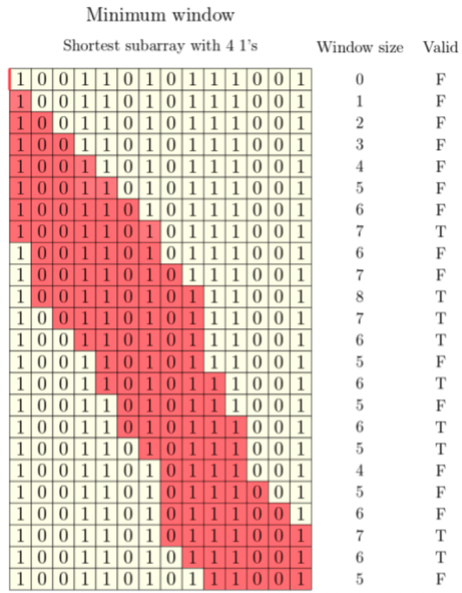
Each row shows one window in red. We start with an empty window, and we stop when the window is invalid and we cannot grow it anymore. The final answer is 5.
Stacks and queues
Stacks
Remarks
TBD
# declaration (Python list by default)
stack = []
# push
stack.append(1)
stack.append(2)
stack.append(3)
# pop
stack.pop() # 3
stack.pop() # 2
# peek
stack[-1] # 1
# empty check
not stack # False
# size check
len(stack) # 1
Examples
LC 20. Valid Parentheses (✓) ★
Given a string s containing just the characters '(', ')', '{', '}', '[' and ']', determine if the input string is valid.
An input string is valid if:
- Open brackets must be closed by the same type of brackets.
- Open brackets must be closed in the correct order.
class Solution:
def isValid(self, s: str) -> bool:
lookup = {
')': '(',
'}': '{',
']': '['
}
stack = []
for char in s:
if char in lookup:
if not stack or lookup[char] != stack.pop():
return False
else:
stack.append(char)
return not stack
Time: . Each character in the input string is processed, and it takes time to process each individual character.
Space: . If the input string is comprised of only opening delimiters, then the stack will grow to be the size of the input string.
The LIFO pattern exhibited for this problem is the following: The last (most recent) opening delimiter is the first to be deleted.
The "correct" order is determined by whatever the previous opening bracket was. Whenever there is a closing bracket, it should correspond to the most recent opening bracket. We can effectively test for this in an iterative fashion by maintaining a history (stack) of the encountered opening delimiters. As soon as we encounter a closing delimiter, if the element on top of the stack doesn't correspond (or if the stack is empty), then we know we cannot have a list of valid parentheses and we can return False; otherwise, the current character is an opening delimiter and we add it to the stack.
Once we've completed iterating through all characters, if the stack of opening delimiters is empty, then we know all delimiters have a valid correspondence, and we can return True.
LC 1047. Remove All Adjacent Duplicates In String (✓)
Given a string S of lowercase letters, a duplicate removal consists of choosing two adjacent and equal letters, and removing them.
We repeatedly make duplicate removals on S until we no longer can.
Return the final string after all such duplicate removals have been made. It is guaranteed the answer is unique.
class Solution:
def removeDuplicates(self, s: str) -> str:
stack = []
for char in s:
if stack and stack[-1] == char:
stack.pop()
else:
stack.append(char)
return ''.join(stack)
Time: . Each character in the input string is processed, and it takes time to process each character.
Space: . If all characters are unique, then the stack will grow to be the size of the input string.
The LIFO pattern exhibited in this problem is the following: The last (most recent) character is the first to be deleted.
The example of s = "azxxzy" resolving to "ay" highlights the strategy we should use here, namely determining whether or not the current character ever equals the element on top of the stack. If so, then remove the element from the top of the stack and continue on (this effectively deletes both elements); otherwise, add the current element to the stack.
LC 844. Backspace String Compare (✓)
Given two strings s and t, return true if they are equal when both are typed into empty text editors. '#' means a backspace character.
Note that after backspacing an empty text, the text will continue empty.
class Solution:
def backspaceCompare(self, s: str, t: str) -> bool:
def typed_str(r):
stack = []
for char in r:
if char == '#':
if stack:
stack.pop()
else:
stack.append(char)
return ''.join(stack)
return typed_str(s) == typed_str(t)
Time: . Let the lengths of the strings s and t be m and n, respectively. Both strings are processed in a linear fashion, and it takes time to process each character.
Space: . If no backspaces are encountered, then the memory consumed will be proportional to the length of s and t, combined.
The following LIFO property is on display in this problem: Maintaining a history of characters seen and deleting the most recently seen ones when # characters are encountered.
The stack-based solution is quick and easy since # characters almost literally allow us to backspace by removing (deleting) characters from the stack that maintains a history of the characters seen so far. A more complicated but elegant solution is a two-pointer approach.
LC 71. Simplify Path (✓)
Given a string path, which is an absolute path (starting with a slash '/') to a file or directory in a Unix-style file system, convert it to the simplified canonical path.
In a Unix-style file system, a period '.' refers to the current directory, a double period '..' refers to the directory up a level, and any multiple consecutive slashes (i.e. '//') are treated as a single slash '/'. For this problem, any other format of periods such as '...' are treated as file/directory names.
The canonical path should have the following format:
- The path starts with a single slash
'/'. - Any two directories are separated by a single slash
'/'. - The path does not end with a trailing
'/'. - The path only contains the directories on the path from the root directory to the target file or directory (i.e., no period
'.'or double period'..')
Return the simplified canonical path.
class Solution:
def simplifyPath(self, path: str) -> str:
stack = []
for portion in path.split('/'):
if portion == '' or portion == '.':
continue
elif portion == '..':
if stack:
stack.pop()
else:
stack.append(portion)
return '/' + '/'.join(stack)
Time: . It takes time to process all characters in path when executing path.split('/'), and there's also a smaller cost in comparing the portion substrings to pre-defined special character groups (i.e., '', '.', and '..').
Space: . It takes space to aggregate the groups in path.split('/') and space to build the canonical path in stack, resulting in an overall space complexity of .
LIFO property at work in this problem: Only ever add valid file/directory names to the stack. If you encounter .., then remove the most recently seen file or directory name. If you encounter other characters such as '' or '.', then it's a no-op and you should continue on with your processing. At the end, return a string joined with / separators (the first / needs to be manually inserted).
One of the tricks in this problem is to only aggregate directory names as opposed to operations on those directories. The operations dictate how we manage the stack (as alluded to above).
LC 1544. Make The String Great (✓)
Given a string s of lower and upper case English letters.
A good string is a string which doesn't have two adjacent characters s[i] and s[i + 1] where:
0 <= i <= s.length - 2s[i]is a lower-case letter ands[i + 1]is the same letter but in upper-case or vice-versa.
To make the string good, you can choose two adjacent characters that make the string bad and remove them. You can keep doing this until the string becomes good.
Return the string after making it good. The answer is guaranteed to be unique under the given constraints.
Notice that an empty string is also good.
class Solution:
def makeGood(self, s: str) -> str:
stack = []
for char in s:
if stack and abs(ord(stack[-1]) - ord(char)) == 32:
stack.pop()
else:
stack.append(char)
return ''.join(stack)
Time: . The entire input string is processed, and it takes time to process each character individually.
Space: . The stack size could become as large as the input string itself.
The LIFO property at work in this problem: The last character added to the stack is the first one out if its corresponding upper- or lower-case character is the one currently being considered.
LC 2390. Removing Stars From a String (✓)
You are given a string s, which contains stars *.
In one operation, you can:
- Choose a star in
s. - Remove the closest non-star character to its left, as well as remove the star itself.
Return the string after all stars have been removed.
Note:
- The input will be generated such that the operation is always possible.
- It can be shown that the resulting string will always be unique.
class Solution:
def removeStars(self, s: str) -> str:
stack = []
for i in range(len(s)):
if s[i] == '*' and stack:
stack.pop()
else:
stack.append(s[i])
return "".join(stack)
LC 232. Implement Queue using Stacks (✓) ★★
Implement a first in first out (FIFO) queue using only two stacks. The implemented queue should support all the functions of a normal queue (push, peek, pop, and empty).
Implement the MyQueue class:
void push(int x)Pushes element x to the back of the queue.int pop()Removes the element from the front of the queue and returns it.int peek()Returns the element at the front of the queue.boolean empty()Returnstrueif the queue is empty,falseotherwise.
Notes:
- You must use only standard operations of a stack, which means only
push to top,peek/pop from top,size, andis emptyoperations are valid. - Depending on your language, the stack may not be supported natively. You may simulate a stack using a list or deque (double-ended queue) as long as you use only a stack's standard operations.
Follow-up: Can you implement the queue such that each operation is amortized O(1) time complexity? In other words, performing n operations will take overall O(n) time even if one of those operations may take longer.
class MyQueue:
def __init__(self):
self.enqueued = []
self.dequeue = []
self.front = None
def push(self, x: int) -> None:
if not self.enqueued:
self.front = x
self.enqueued.append(x)
def pop(self) -> int:
if not self.dequeue:
while self.enqueued:
self.dequeue.append(self.enqueued.pop())
if self.dequeue:
return self.dequeue.pop()
def peek(self) -> int:
if not self.dequeue:
return self.front
else:
return self.dequeue[-1]
def empty(self) -> bool:
return len(self.enqueued) == 0 and len(self.dequeue) == 0
The main insight for solving this problem performantly is realizing that, since stacks are LIFO (last in first out), this means elements popped from the stack appear in reverse order compared to how they were entered. For example, suppose the values 1, 2, and 3 are pushed to a stack. Then popping them off one at a time yields 3, 2, and 1, in that order.
Hence, to start, we just keep pushing elements to a stack, self.enqueued. These are the elements that have been enqueued so far. As soon as we need to pop an element from the queue, this means we need to access and remove the element at the bottom of the self.enqueued stack. To do this, we use another stack, self.dequeue, to collect the values from self.enqueued in reverse order. The element to be popped from the queue is now at the top of the self.dequeue stack.
This strategy works beyond just a way "to start". Since all of the elements in self.dequeue are the elements originally in self.enqueued but reversed, this means we can pop an element from self.dequeue whenever we're asked to pop an element from the queue. So long as self.dequeue isn't empty! If, however, self.dequeue, is empty, then we'll need to again pop all the elements from self.enqueued so that self.dequeue will contain the elements in proper FIFO order.
The process outlined above for maintaining these stacks is the core of this question, but being able to effectively "peek" from the queue is also a problem worth mentioning. If self.dequeue is not empty, then peeking should simply be the element we would otherwise pop from the queue, which is the element at the top of the self.dequeue stack (we're using the "stack peek" operation in this case): self.dequeue[-1]. But what if self.dequeue is actually empty and we've just been pushing elements to the self.enqueued stack? The element we want is at self.enqueued[0], but accessing the element in this way is not a valid stack operation -- the element is at the bottom of the stack! The idea is to use another class variable, self.front, to keep track of whatever value is at the bottom of self.enqueued (i.e., bottom of this stack or front of the queue). We keep track of this by reassigning self.front whenever we're about to push an element to self.enqueued but self.enqueued is empty. This is how we can keep pushing elements to self.enqueued without losing the reference to the element at the front/bottom. Then, once we're asked to perform a "queue peek" operation, we can either return the element at the top of the self.dequeue stack if it's not empty or self.front if self.dequeue is empty.
LC 2434. Using a Robot to Print the Lexicographically Smallest String (✓) ★
You are given a string s and a robot that currently holds an empty string t. Apply one of the following operations until s and t are both empty:
- Remove the first character of a string
sand give it to the robot. The robot will append this character to the stringt. - Remove the last character of a string
tand give it to the robot. The robot will write this character on paper.
Return the lexicographically smallest string that can be written on the paper.
Approach 1 (frequency array and smallest remaining character helper function)
class Solution:
def robotWithString(self, s: str) -> str:
def smallest_remaining_char(freqs_arr):
for i in range(len(freqs_arr)):
if freqs_arr[i] != 0:
return chr(a_ORD + i)
return 'z'
a_ORD = 97 # ord('a') = 97, the ordinal value of 'a'
freqs = [0] * 26
for char in s:
freqs[ord(char) - a_ORD] += 1
t = []
p = []
for char in s:
t.append(char)
freqs[ord(t[-1]) - a_ORD] -= 1
while t and t[-1] <= smallest_remaining_char(freqs):
p.append(t.pop())
return "".join(p)
The variable t should almost certainly be a stack that holds a "history" of the characters in s as we iterate through them. It doesn't take long to realize that the main challenge here is figuring out when to push a character onto the output string, p, which is a list of accumulated characters that is strategically assembled to satisfy the "lexicographically smallest" demand. The primary idea in this problem is to only pop characters from the stack t when we're guaranteed that doing so enables us to proceed in assembling the lexicographically smallest string.
When, then, should we pop a character from t? Only when there are no remaining characters that are lexicographically smaller than the character on top of the stack t. This means we need some kind of lookup. A lookup for what? The smallest character remaining from wherever we are in our process of iterating through all characters of s. To do this effectively, we need to keep a frequency count (the smallest character remaining at one point could get removed and there could subsequently be more of the same characters to take its place), which is most often done using a hash map. We could do that here, but using a frequency array is arguably cleaner since the characters we care about are 'a' through 'z', meaning our frequency array only needs to have 26 slots.
We assemble the frequency array as our first pass in our solution. The smallest_remaining_char function will always give us the current smallest remaining character from wherever we are when processing the string s (it's helpful to know that 'a''s ordinal value is 97, which we can helpfully use to maintain our frequency array).
Now, each time we process a character from s, we push it to the stack t, and decrement its count from the frequency array, freqs. All that really remains is to proceed as alluded to above, namely pop elements from t into p that are smaller or equal to the smallest element remaining in s.
Approach 2 (minimum remaining character lookup array, no frequency count)
class Solution:
def robotWithString(self, s: str) -> int:
n = len(s)
t = []
p = []
min_char = [s[-1]] * n
for i in range(n - 2, -1, -1):
min_char[i] = min(s[i], min_char[i + 1])
idx = 1
for char in s:
t.append(char)
while idx < n and t and t[-1] <= min_char[idx]:
p.append(t.pop())
idx += 1
while t:
p.append(t.pop())
return "".join(p)
The solution in Approach 1 was whereas the solution above is . The constant factor is much smaller even though both solutions belong to the same efficiency class. Regardless, the solution above still uses the main idea from Approach 1, namely we only ever pop characters from t when they're (lexicographically) smaller or equal to the characters remaining in s. The difference in this approach compared to that in Approach 1 is that we do not use a frequency count; instead, we precompute what the remaining minimum character will be from any character index in s:
min_char = [s[-1]] * n
for i in range(n - 2, -1, -1):
min_char[i] = min(s[i], min_char[i + 1])
This is easiest to understand by means of an example. Suppose we had s = 'laptop'. Then min_char, after running the code above, would yield ['a', 'a', 'o', 'o', 'o', 'p']; that is, at index i = 0, the lexicographically smallest remaining character is 'a'. At position i = 1, the lexicographically smallest remaining character is also 'a'. At index i = 2, the lexicographically smallest remaining character is 'o'. And so forth. This allows us to effectively use the min_char array to determine when elements should be popped from t and placed in p.
LC 946. Validate Stack Sequences (✓) ★
Given two sequences pushed and popped with distinct values, return true if and only if this could have been the result of a sequence of push and pop operations on an initially empty stack.
class Solution(object):
def validateStackSequences(self, pushed, popped):
pop_p = 0
ref = []
for num in pushed:
ref.append(num)
while ref and pop_p < len(popped) and ref[-1] == popped[pop_p]:
ref.pop()
pop_p += 1
return pop_p == len(popped)
The key idea here is somewhat difficult to intuit at first. Basically, we're trying to see if the values in pushed have been pushed (with unspecified pops along the way) in such a way that the pops specified in popped is actually possible; that is, it's almost as if we're starting with an empty stack, and then we proceed to push values into the stack in the order in which they appear in pushed, and along the way, we intermittently pop values from the stack, where the order in which values are popped is preserved in popped.
Hence, one possible strategy is to keep a reference or history of values pushed so far. The LIFO nature of keeping a history naturally suggests a stack. We'll call it ref. Then we can basically iterate through all values in pushed, adding them to the ref stack until the element at the top of the ref stack equals the first element in popped. This means we should pop the value from ref, and it also means we need to move to the second or next value in popped. This way of keeping a reference to values in popped suggests usage of a pointer, pop_p in the solution code above.
We should keep popping elements from ref so long as they match the ones in popped. We only move on to the next value in pushed once this has been done. Our endpoint will naturally be when ref is exhausted and pop_p == len(popped) (this means the sequence specified is possible). If pop_p != len(popped), then this means not all values in popped were accounted for and thus the specification is not possible.
Note: The condition pop_p < len(popped) in the while loop is not strictly necessary since we're guaranteed that pushed is a permutation of popped and hence the same length. The condition pop_p < len(popped) is only ever violated once ref is empty and hence redundant; if, however, pushed were not necessarily a permutation of popped, then pop_p < len(popped) would be necessary (e.g., pushed = [1,2,3,4,5,6,7], popped = [5,6]). Nonetheless, it's best for the sake of clarity to leave this condition in (gains are minimal when excluding the condition).
LC 735. Asteroid Collision (✓)
We are given an array asteroids of integers representing asteroids in a row.
For each asteroid, the absolute value represents its size, and the sign represents its direction (positive meaning right, negative meaning left). Each asteroid moves at the same speed.
Find out the state of the asteroids after all collisions. If two asteroids meet, the smaller one will explode. If both are the same size, both will explode. Two asteroids moving in the same direction will never meet.
class Solution:
def asteroidCollision(self, asteroids: List[int]) -> List[int]:
history = []
for asteroid in asteroids:
history.append(asteroid)
while len(history) > 1 and history[-2] > 0 and history[-1] < 0:
prev = history[-2]
curr = history[-1]
if prev > abs(curr):
history.pop()
elif prev < abs(curr):
curr = history.pop()
history.pop()
history.append(curr)
else:
history.pop()
history.pop()
return history
The main challenge here is to implement the solution in as clean a manner as possible. The actual problem statement is simple enough, but laying out the solution carefully takes a bit of thought:
- We should maintain a history of all asteroids we've seen. It only makes sense to consider removing asteroids from the history if the history has more than a single asteroid, hence the while loop condition
len(history) > 1. - Since we'll be processing asteroids from left to right, asteroid collisions can only happen when the last asteroid in the history is going right and the current asteroid is going left; hence, we have the following condition after adding the current asteroid to the history:
history[-2] > 0 and history[-1] < 0. - Finally, we can proceed with handling the core conditions of the problem:
- If the previous asteroid has a greater size than the current one, then the current asteroid gets exploded (i.e., removed from the history).
- If, however, the previous asteroid's size is actually smaller than the current one, then the previous asteroid needs to be removed. But the current one is at the top of the history; hence, we temporarily remove the top of the history in order to remove the previous asteroid that exploded (then we add the current asteroid back).
- The only other possibility would be for the asteroids to have the same size, in which case both asteroids explode, and they should both be removed from the history.
LC 155. Min Stack (✓)
Design a stack that supports push, pop, top, and retrieving the minimum element in constant time.
Implement the MinStack class:
MinStack()initializes the stack object.void push(val)pushes the elementvalonto the stack.void pop()removes the element on the top of the stack.int top()gets the top element of the stack.int getMin()retrieves the minimum element in the stack.
class MinStack:
def __init__(self):
self.stack = []
self.min_stack = []
def push(self, val: int) -> None:
self.stack.append(val)
if not self.min_stack:
self.min_stack.append(val)
else:
curr_min = self.min_stack[-1]
self.min_stack.append(min(val, curr_min))
def pop(self) -> None:
self.stack.pop()
self.min_stack.pop()
def top(self) -> int:
return self.stack[-1]
def getMin(self) -> int:
return self.min_stack[-1]
The requirement is to implement a solution with time complexity for each function (i.e., push, pop, top, and getMin), and this is a hint in itself. All stacks would generally be designed to make it possible for us to get the minimum (or maximum) if there were no tradeoffs. Of course there must be a tradeoff here, notably one of space. So how should we use space to make each function , particularly the getMin function?
The answer is to maintain two stacks, the stack itself, self.stack, as well as a stack that only keeps track of the minimums so far, self.min_stack. This allows us to keep the stacks in lockstep and to perform normal stack operations as desired while at the same time making it easy to get minimums in time.
Queues
Remarks
TBD
import collections
# declaration (Python deque from collections module)
queue = collections.deque()
# initialize with values (optional)
queue = collections.deque([1, 2, 3])
# enqueue
queue.append(4)
queue.append(5)
# dequeue
queue.popleft() # 1
queue.popleft() # 2
# peek left (next element to be removed)
queue[0] # 3
# peek right
queue[-1] # 5
# empty check
not queue # False
# size check
len(queue) # 3
Examples
LC 933. Number of Recent Calls (✓)
You have a RecentCounter class which counts the number of recent requests within a certain time frame.
Implement the RecentCounter class:
RecentCounter()Initializes the counter with zero recent requests.int ping(int t)Adds a new request at timet, wheretrepresents some time in milliseconds, and returns the number of requests that has happened in the past3000milliseconds (including the new request). Specifically, return the number of requests that have happened in the inclusive range[t - 3000, t].
It is guaranteed that every call to ping uses a strictly larger value of t than the previous call.
class RecentCounter:
def __init__(self):
self.queue = deque()
def ping(self, t: int) -> int:
self.queue.append(t)
while self.queue[-1] < t - 3000:
self.queue.popleft()
return len(self.queue)
Time: . This is due to the fact that a total of t - (t - 3000) + 1 = 3001 elements can be in the range [t - 3000, t], which means the loop in ping may fire up to 3000 times in the worst case, which is a constant.
Space: . The max size of the queue is 3001, as noted above, which is a constant.
The most recently added element will automatically be part of the number of "recent" calls. To determine all recent calls, we need to remove the previous calls not within the specified range of [t - 3000, t]. A queue is the right data structure for this.
LC 346. Moving Average from Data Stream (✓)
Given a stream of integers and a window size, calculate the moving average of all integers in the sliding window.
Implement the MovingAverage class:
MovingAverage(int size)Initializes the object with the size of the windowsize.double next(int val)Returns the moving average of the lastsizevalues of the stream.
class MovingAverage:
def __init__(self, size: int):
self.queue = deque()
self.queue_sum = 0
self.size = size
def next(self, val: int) -> float:
self.queue.append(val)
self.queue_sum += val
if len(self.queue) > self.size:
self.queue_sum -= self.queue.popleft()
return self.queue_sum / len(self.queue)
Time: . The data stream is moving, which means we never process elements in aggregate.
Space: . Let represent the size of the moving window. This is the maximum space consumed in the solution above.
There's nothing to prevent us from keeping track of the total window sum, which we can effectively use the queue to adjust by subtracting elements out of the window (first in first out) and adding new elements to the window.
LC 225. Implement Stack using Queues (✓) ★★
Implement a last in first out (LIFO) stack using only two queues. The implemented stack should support all the functions of a normal queue (push, top, pop, and empty).
Implement the MyStack class:
void push(int x)Pushes element x to the top of the stack.int pop()Removes the element on the top of the stack and returns it.int top()Returns the element on the top of the stack.boolean empty()Returnstrueif the stack is empty,falseotherwise.
Notes:
- You must use only standard operations of a queue, which means only
push to back,peek/pop from front,size, andis emptyoperations are valid. - Depending on your language, the queue may not be supported natively. You may simulate a queue using a list or deque (double-ended queue), as long as you use only a queue's standard operations.
The main idea in each approach below is effectively to "rotate" elements in some way so that the most recent element added is accessible from the front (since we can only pop elements in a queue from the first given its FIFO nature). Approach 1 is the intended solution on LeetCode (and probably what would be acceptable in an interview), but approaches 2 and 3 offer seam neat insights for clever optimizations.
Approach 1 (one queue, O(n) pushes with self-rotations)
class MyStack:
def __init__(self):
self.queue = deque()
def push(self, x: int) -> None:
self.queue.append(x)
size = len(self.queue)
while size > 1:
self.queue.append(self.queue.popleft())
size -= 1
def pop(self) -> int:
return self.queue.popleft()
def top(self) -> int:
return self.queue[0]
def empty(self) -> bool:
return len(self.queue) == 0
The key to solving a similar problem, namely LC 232. Implement Queue using Stacks, was to take advantage of the fact that popping elements from a stack meant obtaining them in reverse order compared to how they are added to the stack. This meant we could use two stacks effectively to simulate a queue, where we kept adding elements to one stack (the "enqueued" stack) and we'd pop elements from the other stack (the "dequeue" stack) once a dequeue operation was requested — the main trick was that we only popped all the elements from the "enqueued" stack to "dequeue" stack when a dequeue operation was requested and the dequeue stack was empty. This meant we could perform the operation in amortized . That's not the case here.
Queues are FIFO so popping elements from the left in one queue and appending them to the right in another queue means elements would be added to the second queue in the same order they were added to the first queue. That is definitely not desirable. The main trick for this problem, which is easy to miss at first because it seems like there must be a more performant way to accomplish this (see Approach 2), is to use a single queue and rotate elements through the queue every time a new element is added so that the new element becomes the left-most element of the queue. Each "push" operation for the stack we're trying to implement requires appending an element to the queue and then rotating through all elements by popping from the left and appending the popped element to the right until the newly added element is the left-most element. For example, consider how the numbers 2, 7, 8, 4 would be added to the queue to simulate a stack:
# first element (2) pushed
[2]
# second element (7) pushed
[2] # start state
[2,7] # 7 gets pushed
[7,2] # 2 gets popped from the left and pushed to the right
# third element (8) pushed
[7,2] # start state
[7,2,8] # 8 gets pushed
[2,8,7] # 7 gets popped from the left and pushed to the right
[8,7,2] # 2 gets popped from the left and pushed to the right
# fourth element (4) pushed
[8,7,2] # start state
[8,7,2,4] # 4 gets pushed
[7,2,4,8] # 8 gets popped from the left and pushed to the right
[2,4,8,7] # 7 gets popped from the left and pushed to the right
[4,8,7,2] # 2 gets popped from the left and pushed to the right
Each push operation for the stack ultimately results in all elements being stored in the deque in reverse order, which is the desired effect. The push operation costs and is really the only complicated operation, but it can be a head scratcher if you haven't seen it before.
Approach 2 (two queues, amortized O(sqrt(n)) pushes with self-rotations and cache)
class MyStack:
def __init__(self):
self.cache = deque()
self.storage = deque()
def push(self, x: int) -> None:
self.cache.append(x)
size = len(self.cache)
while size > 1:
self.cache.append(self.cache.popleft())
size -= 1
if len(self.cache) * len(self.cache) > len(self.storage):
while self.storage:
self.cache.append(self.storage.popleft())
self.cache, self.storage = self.storage, self.cache
def pop(self) -> int:
if self.cache:
return self.cache.popleft()
else:
return self.storage.popleft()
def top(self) -> int:
if self.cache:
return self.cache[0]
else:
return self.storage[0]
def empty(self) -> bool:
return len(self.cache) == 0 and len(self.storage) == 0
The approach above is based on this solution. The core idea of maintaining stack order by rotating through elements is still present from Approach 1. But it seemed like there must be a more performant way to push elements to our stack than requiring an approach every time (i.e., rotating through all elements for each push).
The core of the solution above is the same as that in Approach 1 (i.e., rotating through elements), but now we're effectively trying to reduce the amount of rotating we have to do for each push. The idea is to maintain two queues, one that acts as a cache and one that acts as main storage. How does this help? Costly rotations arising from push operations will only be executed on the cache, and our goal will be to keep the size of cache small. When the size of cache exceeds the square root of the size of storage, the following will happen:
- All of the elements in
storagewill be popped and appended tocache. - The variable designations will be swapped so now
cacheis empty andstoragehas all elements in the stack.
Important to note is that both cache and storage will always be maintained in LIFO order, with cache holding the newest elements at the top of the stack and storage holding the oldest. An example that illustrates the mechanics of how this works will be most helpful. Suppose we're trying to push the following elements to our stack: 1, 2, 3, 4, 5, 6, 7, 8. This is how the process would look:
##### PUSHING (1)
cache = [] # start state
storage = [] # start state
cache = [1] # after adding 1
storage = []
# len(cache) * len(cache) = 1 * 1 = 1 > 0 = len(storage) [YES, transfer and reassign]
# self.storage is empty so the empty pop doesn't happen: self.cache.append(self.storage.popleft())
# we still end up swapping/reassigning cache and storage
cache = []
storage = [1]
##### PUSHING (2)
cache = [] # start state
storage = [1]
cache = [2] # after pushing 2
storage = [1]
# len(cache) * len(cache) = 1 * 1 = 1 > 1 = len(storage) [NO, terminate push op]
##### PUSHING (3)
cache = [2] # start state
storage = [1]
cache = [2,3] # after pushing 3
cache = [3,2] # after rotating
storage = [1]
# len(cache) * len(cache) = 2 * 2 = 4 > 1 = len(storage) [YES, transfer and reassign]
cache = [3,2,1] # pop left all elements in storage and append to cache
storage = [] # pop ALL elements from storage from the left and append to cache until empty
cache = [] # swap and reassign
storage = [3,2,1]
##### PUSHING (4)
cache = [] # start state
storage = [3,2,1]
cache = [4] # after pushing 4
storage = [3,2,1]
# len(cache) * len(cache) = 1 * 1 = 1 > 3 = len(storage) [NO, terminate push op]
##### PUSHING (5)
cache = [4] # start state
storage = [3,2,1]
cache = [4,5] # after pushing 5
cache = [5,4] # after rotating
storage = [3,2,1]
# len(cache) * len(cache) = 2 * 2 = 4 > 3 = len(storage) [YES, transfer and reassign]
cache = [5,4,3,2,1] # pop left all elements in storage and append to cache
storage = [] # pop ALL elements from storage from the left and append to cache until empty
cache = [] # swap and reassign
storage = [5,4,3,2,1]
##### PUSHING (6)
cache = [] # start state
storage = [5,4,3,2,1]
cache = [6] # after pushing 6
storage = [5,4,3,2,1]
# len(cache) * len(cache) = 1 * 1 = 1 > 5 = len(storage) [NO, terminate push op]
##### PUSHING (7)
cache = [] # start state
storage = [5,4,3,2,1]
cache = [6,7] # after pushing 7
cache = [7,6] # after rotating
storage = [5,4,3,2,1]
# len(cache) * len(cache) = 2 * 2 = 4 > 5 = len(storage) [NO, terminate push op]
##### PUSHING (8)
cache = [7,6] # start state
storage = [5,4,3,2,1]
cache = [7,6,8] # after pushing 8
cache = [8,7,6] # after rotating
storage = [5,4,3,2,1]
# len(cache) * len(cache) = 3 * 3 = 6 > 5 = len(storage) [YES, transfer and reassign]
cache = [8,7,6,5,4,3,2,1] # pop left all elements in storage and append to cache
storage = [] # pop ALL elements from storage from the left and append to cache until empty
cache = [] # swap and reassign
storage = [8,7,6,5,4,3,2,1]
The mechanics of the process illustrated above show how cache always maintains the top elements of the stack until its size limit (the square root of the size of storage) has been exceeded. Then all elements from storage are transfered to cache so as to maintain the LIFO order of the stack. Then cache and storage are swapped/reassigned so that cache is now empty again. Hence, storage is the main storage for the stack and keeps growing indefinitely while cache, on the other hand, is sort of an intermediary device that's used to make sure storage grows in size as efficient as possible.
As this post notes:
pushworks in amortized time. There are two cases: if , thenpushtakes time. If , thenpushtakes time, but after this operationcachewill be empty. It will take time before we get to this case again, so the amortized time is time.
Approach 3 (dynamic number of deques, O(1) operations)
class MyStack:
def __init__(self):
self.queue = deque()
def push(self, x: int) -> None:
new_queue = deque()
new_queue.append(x)
new_queue.append(self.queue)
self.queue = new_queue
def pop(self) -> int:
pop_val = self.queue.popleft()
self.queue = self.queue.popleft()
return pop_val
def top(self) -> int:
return self.queue[0]
def empty(self) -> bool:
return len(self.queue) == 0
The solution above, inspired by Stefan Pochmann's, shows it is possible to implement MyStack using only operations if we get really creative (even though this may be thought of as "cheating" in some sense because we use an unlimited number of deques). This solution takes advantage of the fact that Python is fundamentally a reference-based language: adding a queue object into another does not copy the entire contents — this is an operation since a linked list is used under the hood (for Python deques).
To illustrate exactly how and why the solution above works, considering pushing the following elements to our stack: 1, 2, 3. Below, we'll let D represent a deque collection:
# starting state
self.queue = D()
# pushing 1
new_queue = D(1) # after pushing 1
= D(1, D()) # after pushing self.queue
self.queue = D(1, D()) # end state after pushing x
# pushing 2
new_queue = D(2) # after pushing 2
= D(2, D(1, D())) # after pushing self.queue
self.queue = D(2, D(1, D())) # end state after pushing 2
# pushing 3
new_queue = D(3) # after pushing 3
= D(3, D(2, D(1, D()))) # after pushing self.queue
self.queue = D(3, D(2, D(1, D()))) # end state after pushing 3
The process illustrated above shows how we always have access to the most recently added element (desirable for stacks because of the LIFO processing). Popping an element is also easy. Consider the final state of the example above: popping an element from the left (a queue operation) of self.queue means popping the left-most element of D(3, D(2, D(1, D()))), which is the integer 3, as desired. After this pop, we have self.queue = D(D(2, D(1, D()))), which is not desirable because now if we pop left then we'll get a deque and not an integer, as desired and required. But this is not much of an issue because all we have to do is reassign self.queue to be the left-most popped element (after popping the 3, the deque only consists of one element, the deque with everything else in the stack): self.queue = D(2, D(1, D())). Now we can pop left to get the 2 and reassign by popping left again to get D(1, D()). Finally, we can pop left to get the 1 and reassign by popping left again to end up back where we started: D().
LC 649. Dota2 Senate (✓)
In the world of Dota2, there are two parties: the Radiant and the Dire.
The Dota2 senate consists of senators coming from two parties. Now the senate wants to make a decision about a change in the Dota2 game. The voting for this change is a round-based procedure. In each round, each senator can exercise one of the two rights:
Ban one senator's right: A senator can make another senator lose all his rights in this and all the following rounds.Announce the victory: If this senator found the senators who still have rights to vote are all from the same party, he can announce the victory and make the decision about the change in the game.
Given a string representing each senator's party belonging. The character 'R' and 'D' represent the Radiant party and the Dire party respectively. Then if there are n senators, the size of the given string will be n.
The round-based procedure starts from the first senator to the last senator in the given order. This procedure will last until the end of voting. All the senators who have lost their rights will be skipped during the procedure.
Suppose every senator is smart enough and will play the best strategy for his own party, you need to predict which party will finally announce the victory and make the change in the Dota2 game. The output should be Radiant or Dire.
class Solution:
def predictPartyVictory(self, senate: str) -> str:
n = len(senate)
r_sen = deque()
d_sen = deque()
for i in range(len(senate)):
if senate[i] == 'R':
r_sen.append(i)
else:
d_sen.append(i)
while r_sen and d_sen:
banning, banned = min(r_sen[0], d_sen[0]), max(r_sen[0], d_sen[0])
if r_sen[0] == banning:
r_sen.append(r_sen.popleft() + n)
d_sen.popleft()
else:
d_sen.append(d_sen.popleft() + n)
r_sen.popleft()
return 'Radiant' if len(r_sen) > 0 else 'Dire'
This is quite the difficult problem, one where using queues is not at all obvious at first. The solution above (not due to me) is quite brilliant. The core idea, which will be reinforced/illustrated by means of an example in just a moment, is to create two queues, one for each set of senators. Why?
We can safely assume that senators will always act in a greedy way (i.e., they will always ban the senator of the opposing party if there is one). How do we know how to keep track of the senators and their banning decisions? Without queues, that becomes a more difficult question to answer. With queues, however, this becomes a much more straightforward question: we do a first pass of senate and assemble queues of indexes for both parties, the Radiant senators, r_sen, and the Dire senators d_sen.
While both queues are non-empty, we compare their leftmost entries. Indexes naturally correspond to positions for the senators (i.e., the smaller index comes first); hence, the senator with the smaller index of the two will be the senator who does the banning while the senator with the larger of the indexes gets banned. The banned senator can simply be popped from the queue (popped from the left), but the senator who does the banning will have to wait for the next round (given the problem's circular nature). A clever solution to ensure the senator who does the banning is actually involved in the next round is to pop the banning senator from the queue (pop left), and then to push that same senator to the back of the same queue but this time with a larger index to indicate this senator comes later. The easiest way to adroitly perform this index manipulation is just by adding n to the index that already exists, where n is the size of the original senate string.
Whichever queue ends up being non-empty is the victorious senate party.
Note: As can be seen in the solution above, we don't actually need to declare the banned variable. We can remove it without issue since it is not used (it was only included to illustrate the explanation above).
Monotonic stacks
Remarks
See the monotonic stack blog post for more on gaining an intuition for monotonic stacks and deques.
Old examples
LC 739. Daily Temperatures (✓)
Given an array of integers temperatures that represents the daily temperatures, return an array answer such that answer[i] is the number of days you have to wait after the ith day to get a warmer temperature. If there is no future day for which this is possible, keep answer[i] == 0 instead.
class Solution:
def dailyTemperatures(self, temperatures: List[int]) -> List[int]:
n = len(temperatures)
ans = [None] * n
stack = []
for i in range(n):
val_A = temperatures[i]
# try to find the next larger temperature, val_B,
# for the current temperature, val_A
while stack and temperatures[stack[-1]] < val_A:
idx_val_B = stack.pop()
ans[idx_val_B] = i - idx_val_B
stack.append(i)
# remaining temperatures, val_A, have no next larger temperature, val_B
while stack:
idx_val_A = stack.pop()
ans[idx_val_A] = 0
return ans
See the blog post on monotonic stacks and queues for a more in depth discussion of the solution above, if needed.
LC 239. Sliding Window Maximum (✓)
You are given an array of integers nums, there is a sliding window of size k which is moving from the very left of the array to the very right. You can only see the k numbers in the window. Each time the sliding window moves right by one position.
Return the max sliding window.
class Solution:
def maxSlidingWindow(self, nums: List[int], k: int) -> List[int]:
n = len(nums)
dec_queue = deque() # monotonic deque (weakly decreasing)
ans = []
for i in range(n):
curr_num = nums[i]
# maintain the weakly decreasing deque
while dec_queue and nums[dec_queue[-1]] < curr_num:
dec_queue.pop()
# check to see if leftmost value of the deque
# is now actually an invalid index
if dec_queue and dec_queue[0] == i - k:
dec_queue.popleft()
dec_queue.append(i)
# only add window maximums to the answer array
# once the required length has been reached
if i >= k - 1:
ans.append(nums[dec_queue[0]])
return ans
See the blog post on monotonic stacks and queues for a more in depth discussion of the solution above, if needed.
LC 1438. Longest Continuous Subarray With Absolute Diff Less Than or Equal to Limit (✓)
Given an array of integers nums and an integer limit, return the size of the longest non-empty subarray such that the absolute difference between any two elements of this subarray is less than or equal to limit.
class Solution:
def longestSubarray(self, nums: List[int], limit: int) -> int:
n = len(nums)
dec_queue = deque() # monotonic deque (weakly decreasing) for the maximums
inc_queue = deque() # monotonic deque (weakly increasing) for the minimums
left = ans = 0
for right in range(n):
curr_num = nums[right]
# maintain the deque invariants
while dec_queue and nums[dec_queue[-1]] < curr_num:
dec_queue.pop()
while inc_queue and nums[inc_queue[-1]] > curr_num:
inc_queue.pop()
dec_queue.append(right)
inc_queue.append(right)
# update sliding window to ensure the window is valid
while left <= right and nums[dec_queue[0]] - nums[inc_queue[0]] > limit:
# remove possibly invalidated indexes from the deques once the window has shifted
if dec_queue[0] == left:
dec_queue.popleft()
if inc_queue[0] == left:
inc_queue.popleft()
left += 1
# update the answer with the length of the current valid window
ans = max(ans, right - left + 1)
return ans
See the blog post on monotonic stacks and queues for a more in depth discussion of the solution above, if needed.
LC 496. Next Greater Element I (✓)
You are given two integer arrays nums1 and nums2 both of unique elements, where nums1 is a subset of nums2.
Find all the next greater numbers for nums1's elements in the corresponding places of nums2.
The Next Greater Number of a number x in nums1 is the first greater number to its right in nums2. If it does not exist, return -1 for this number.
class Solution:
def nextGreaterElement(self, nums1: List[int], nums2: List[int]) -> List[int]:
queries = {}
stack = []
# determine "next greater" values in nums2
for i in range(len(nums2)):
val_B = nums2[i]
while stack and nums2[stack[-1]] < val_B:
idx_val_A = stack.pop()
val_A = nums2[idx_val_A]
queries[val_A] = val_B
stack.append(i)
# remaining values have no next greater value (default to -1)
while stack:
idx_val_A = stack.pop()
val_A = nums2[idx_val_A]
queries[val_A] = -1
# the queries hash map tells us the next greater value
# for each value queried from nums1
ans = [None] * len(nums1)
for i in range(len(nums1)):
ans[i] = queries[nums1[i]]
return ans
See the blog post on monotonic stacks and queues for a more in depth discussion of the solution above, if needed.
LC 503. Next Greater Element II
Given a circular integer array nums (i.e., the next element of nums[nums.length - 1] is nums[0]), return the next greater number for every element in nums.
The next greater number of a number x is the first greater number to its traversing-order next in the array, which means you could search circularly to find its next greater number. If it doesn't exist, return -1 for this number.
class Solution:
def nextGreaterElements(self, nums: List[int]) -> List[int]:
n = len(nums)
ans = [None] * n
stack = []
for i in range(n * 2):
val_B = nums[i % n]
while stack and nums[stack[-1]] < val_B:
idx_val_A = stack.pop()
ans[idx_val_A] = val_B
# only add elements to the stack on the first full pass
if i < n:
stack.append(i)
else:
# otherwise the remaining values (if there are any)
# never had a next greater element; hence, we simply
# make another full pass to see if any element is greater
# than the current element in the stack and then pop the
# element from the stack if the answer is affirmative
if stack and nums[stack[-1]] < nums[i % n]:
idx_val_A = stack.pop()
ans[idx_val_A] = nums[i % n]
# the remaining values in the stack are those that do not have a next
# greater element despite two full passes; we report -1 for these values
while stack:
idx_val_A = stack.pop()
ans[idx_val_A] = -1
return ans
See the blog post on monotonic stacks and queues for a more in depth discussion of the solution above, if needed.
LC 901. Online Stock Span (✓)
Write a class StockSpanner which collects daily price quotes for some stock, and returns the span of that stock's price for the current day.
The span of the stock's price today is defined as the maximum number of consecutive days (starting from today and going backwards) for which the price of the stock was less than or equal to today's price.
For example, if the price of a stock over the next 7 days were [100, 80, 60, 70, 60, 75, 85], then the stock spans would be [1, 1, 1, 2, 1, 4, 6].
class StockSpanner:
def __init__(self):
self.stack = []
self.idx = 0
def next(self, price: int) -> int:
val_A = price
while self.stack and self.stack[-1][0] <= price:
self.stack.pop()
if self.stack:
idx_val_B = self.stack[-1][1]
val_B = self.stack[-1][0]
stock_span = self.idx - idx_val_B
else:
stock_span = self.idx + 1
self.stack.append([val_A, self.idx])
self.idx += 1
return stock_span
See the blog post on monotonic stacks and queues for a more in depth discussion of the solution above, if needed.
LC 1475. Final Prices With a Special Discount in a Shop (✓)
Given the array prices where prices[i] is the price of the ith item in a shop. There is a special discount for items in the shop, if you buy the ith item, then you will receive a discount equivalent to prices[j] where j is the minimum index such that j > i and prices[j] <= prices[i], otherwise, you will not receive any discount at all.
Return an array where the ith element is the final price you will pay for the ith item of the shop considering the special discount.
class Solution:
def finalPrices(self, prices: List[int]) -> List[int]:
n = len(prices)
stack = []
for i in range(n):
val_B = prices[i]
while stack and prices[stack[-1]] >= val_B:
idx_val_A = stack.pop()
prices[idx_val_A] -= val_B # val_B is discount since it is next less or equal value to val_A
stack.append(i)
return prices
See the blog post on monotonic stacks and queues for a more in depth discussion of the solution above, if needed.
LC 1063. Number of Valid Subarrays (✓)
Given an array A of integers, return the number of non-empty continuous subarrays that satisfy the following condition:
The leftmost element of the subarray is not larger than other elements in the subarray.
class Solution:
def validSubarrays(self, nums: List[int]) -> int:
n = len(nums)
queries = [n] * n
stack = []
ans = 0
for i in range(n):
val_B = nums[i]
while stack and nums[stack[-1]] > val_B:
idx_val_A = stack.pop()
queries[idx_val_A] = i
stack.append(i)
# query the next smaller value for each index of nums
# the current index will be the included left endpoint
# and the queried value will be the excluded right endpoint
# total number of subarrays contributed where the left endpoint
# is the minimum: right - left (since right is excluded)
for left in range(n):
right = queries[left]
ans += right - left # NOT "right - left + 1" because right is not included here
return ans
See the blog post on monotonic stacks and queues for a more in depth discussion of the solution above, if needed.
LC 1673. Find the Most Competitive Subsequence (✓)
Given an integer array nums and a positive integer k, return the most competitive subsequence of nums of size k.
An array's subsequence is a resulting sequence obtained by erasing some (possibly zero) elements from the array.
We define that a subsequence a is more competitive than a subsequence b (of the same length) if in the first position where a and b differ, subsequence a has a number less than the corresponding number in b. For example, [1,3,4] is more competitive than [1,3,5] because the first position they differ is at the final number, and 4 is less than 5.
class Solution:
def mostCompetitive(self, nums: List[int], k: int) -> List[int]:
n = len(nums)
stack = []
for i in range(n):
curr_num = nums[i]
while stack and stack[-1] > curr_num and (n - i + len(stack) > k):
stack.pop()
if len(stack) < k:
stack.append(nums[i])
return stack
See the blog post on monotonic stacks and queues for a more in depth discussion of the solution above, if needed.
LC 1944. Number of Visible People in a Queue (✓)
There are n people standing in a queue, and they numbered from 0 to n - 1 in left to right order. You are given an array heights of distinct integers where heights[i] represents the height of the ith person.
A person can see another person to their right in the queue if everybody in between is shorter than both of them. More formally, the ith person can see the jth person if i < j and min(heights[i], heights[j]) > max(heights[i+1], heights[i+2], ..., heights[j-1]).
Return an array answer of length n where answer[i] is the number of people the ith person can see to their right in the queue.
class Solution:
def canSeePersonsCount(self, heights: List[int]) -> List[int]:
n = len(heights)
ans = [0] * n
stack = [] # monotonic stack (decreasing)
for i in range(n):
curr_height = heights[i]
while stack and heights[stack[-1]] < curr_height:
idx_prev_smaller_height = stack.pop()
ans[idx_prev_smaller_height] += 1
if stack:
ans[stack[-1]] += 1
stack.append(i)
return ans
See the blog post on monotonic stacks and queues for a more in depth discussion of the solution above, if needed.
LC 2398. Maximum Number of Robots Within Budget (✓)
You have n robots. You are given two 0-indexed integer arrays, chargeTimes and runningCosts, both of length n. The ith robot costs chargeTimes[i] units to charge and costs runningCosts[i] units to run. You are also given an integer budget.
The total cost of running k chosen robots is equal to max(chargeTimes) + k * sum(runningCosts), where max(chargeTimes) is the largest charge cost among the k robots and sum(runningCosts) is the sum of running costs among the k robots.
Return the maximum number of consecutive robots you can run such that the total cost does not exceed budget.
class Solution:
def maximumRobots(self, chargeTimes: List[int], runningCosts: List[int], budget: int) -> int:
dec_queue = deque() # monotonic deque (weakly decreasing) for charge times
left = window_sum = ans = 0
for right in range(len(chargeTimes)):
# maintain monotonic deque to ensure maximum charge time in window is quickly accessible
curr_charge = chargeTimes[right]
while dec_queue and chargeTimes[dec_queue[-1]] < curr_charge:
dec_queue.pop()
dec_queue.append(right)
# maintain total running cost of sliding window
curr_running_cost = runningCosts[right]
window_sum += curr_running_cost
while left <= right and dec_queue and chargeTimes[dec_queue[0]] + (right - left + 1) * window_sum > budget:
# adjust window_sum to reflect new sliding window's total running cost
window_sum -= runningCosts[left]
# remove leftmost queue element if index is no longer valid after shifting window
if dec_queue[0] == left:
dec_queue.popleft()
left += 1
ans = max(ans, right - left + 1)
return ans
See the blog post on monotonic stacks and queues for a more in depth discussion of the solution above, if needed.
LC 907. Sum of Subarray Minimums (✓)
Given an array of integers arr, find the sum of min(b), where b ranges over every (contiguous) subarray of arr. Since the answer may be large, return the answer modulo 109 + 7.
class Solution:
def sumSubarrayMins(self, arr: List[int]) -> int:
n = len(arr)
stack = []
ans = 0
MOD = 10 ** 9 + 7
for i in range(n + 1):
while stack and (i == n or arr[stack[-1]] >= arr[i]):
curr_min_idx = stack.pop()
curr_min = arr[curr_min_idx]
left_boundary = -1 if not stack else stack[-1]
right_boundary = i
num_subarrays = (curr_min_idx - left_boundary) * (right_boundary - curr_min_idx)
contribution = curr_min * num_subarrays
ans += contribution
stack.append(i)
return ans % MOD
See the blog post on monotonic stacks and queues for a more in depth discussion of the solution above, if needed.
LC 2104. Sum of Subarray Ranges (✓)
You are given an integer array nums. The range of a subarray of nums is the difference between the largest and smallest element in the subarray.
Return the sum of all subarray ranges of nums.
A subarray is a contiguous non-empty sequence of elements within an array.
class Solution:
def subArrayRanges(self, nums: List[int]) -> int:
n = len(nums)
stack = []
total_subarray_minimum_sum = 0
total_subarray_maximum_sum = 0
# calculate total contribution of subarray minimums
for i in range(n + 1):
while stack and (i == n or nums[stack[-1]] >= nums[i]): # note: either '>=' or '>' can be used
curr_min_idx = stack.pop()
curr_min = nums[curr_min_idx]
left_boundary = -1 if not stack else stack[-1]
right_boundary = i
num_subarrays = (curr_min_idx - left_boundary) * (right_boundary - curr_min_idx)
contribution = curr_min * num_subarrays
total_subarray_minimum_sum += contribution
stack.append(i)
# reset the stack
stack = []
# calculate total contribution of subarray maximums
for i in range(n + 1):
while stack and (i == n or nums[stack[-1]] <= nums[i]): # note: either '<=' or '<' can be used
curr_max_idx = stack.pop()
curr_max = nums[curr_max_idx]
left_boundary = -1 if not stack else stack[-1]
right_boundary = i
num_subarrays = (curr_max_idx - left_boundary) * (right_boundary - curr_max_idx)
contribution = curr_max * num_subarrays
total_subarray_maximum_sum += contribution
stack.append(i)
return total_subarray_maximum_sum - total_subarray_minimum_sum
See the blog post on monotonic stacks and queues for a more in depth discussion of the solution above, if needed.
LC 2487. Remove Nodes From Linked List★★★
You are given the head of a linked list.
Remove every node which has a node with a strictly greater value anywhere to the right side of it.
Return the head of the modified linked list.
class Solution:
def removeNodes(self, head: Optional[ListNode]) -> Optional[ListNode]:
sentinel = ListNode(float('inf'))
sentinel.next = head
curr = head
stack = [sentinel]
while curr:
while stack and stack[-1].val < curr.val:
stack.pop()
stack[-1].next = curr
stack.append(curr)
curr = curr.next
return sentinel.next
For each node, its previous "greater than or equal to" node should be linked to it; that is, maintaining a weakly decreasing monotonic stack gives us what we want by first pushing to it the sentinel node whose value is infinite (positively). This means our stack will never be empty; hence, we do not always need to make the check if stack as we might normally have to otherwise. The pointer manipulation here is really quite clever.
Next values
def fn(nums):
n = len(nums)
ans = [None] * n
stack = [] # monotonic stack
for i in range(n):
val_B = nums[i]
# the comparison operator (?) dictates what A's next value B represents
# (<) next larger value (weakly decreasing stack)
# (<=) next larger or equal value (strictly decreasing stack)
# (>) next smaller value (weakly increasing stack)
# (>=) next smaller or equal value (strictly increasing stack)
while stack and nums[stack[-1]] ? val_B:
idx_val_A = stack.pop()
ans[idx_val_A] = val_B
stack.append(i)
# process elements that never had a "next" value that satisfied the criteria
while stack:
idx_val_A = stack.pop()
ans[idx_val_A] = -1
return ans
Previous values
def fn(nums):
n = len(nums)
ans = [None] * n
stack = [] # monotonic stack
for i in range(n):
val_A = nums[i]
# the comparison operator (?) dictates what A's previous value B represents
# (<) previous larger or equal value (weakly decreasing stack)
# (<=) previous larger (strictly decreasing stack)
# (>) previous smaller or equal value (weakly increasing stack)
# (>=) previous smaller value (strictly increasing stack)
while stack and nums[stack[-1]] ? val_A:
stack.pop()
if stack:
idx_val_B = stack[-1]
val_B = nums[idx_val_B]
ans[i] = val_B
else:
ans[i] = -1
stack.append(i)
return ans
Next and previous values (combined)
def fn(nums):
n = len(nums)
ans = [[-1, -1] for _ in range(n)] # default values for missing PREVIOUS and NEXT values, respectively
stack = [] # monotonic stack
# the comparison operator (?) dictates what each element's PREVIOUS and NEXT values will be
# (<) PREVIOUS larger or equal value and NEXT larger value (weakly decreasing stack)
# (<=) PREVIOUS larger value and NEXT larger or equal value (strictly decreasing stack)
# (>) PREVIOUS smaller or equal value and NEXT smaller value (weakly increasing stack)
# (>=) PREVIOUS smaller value and NEXT smaller or equal value (strictly increasing stack)
for i in range(n):
while stack and nums[stack[-1]] ? nums[i]:
# NEXT values processed
idx = stack.pop()
ans[idx][1] = i # use nums[i] instead of i to directly record array values instead of indexes
# PREVIOUS values processed
ans[i][0] = -1 if not stack else stack[-1] # use nums[stack[-1]] instead of stack[-1]
# to directly record array values instead of indexes
stack.append(i)
return ans
Double-ended queue (deque)
from collections import deque
def fn(nums):
queue = deque() # monotonic deque (weakly decreasing)
ans = []
for i in range(len(nums)):
curr_num = nums[i]
while queue and nums[queue[-1]] < curr_num:
queue.pop()
queue.append(i)
if CONDITION:
queue.popleft()
return ans
Trees
__A______ | Pre-order (L -> R): A B X E M S W T P N C H
/ \ | Pre-order (R -> L): A W C H T N P B S X M E
__B __W__ | Post-order (L -> R): E M X S B P N T H C W A
/ \ / \ | Post-order (R -> L): H C N P T W S M E X B A
X S T C | In-order (L -> R): E X M B S A P T N W H C
/ \ / \ / | In-order (R -> L): C H W N T P A S B M X E
E M P N H | Level-order (L -> R): A B W X S T C E M P N H
| Level-order (R -> L): A W B C T S X H N P M E
Manually determine order of nodes visited ("tick trick")
Tick trick overview
One online resource does a good job of detailing the so-called tick trick, a handy trick for figuring out by hand the order in which a binary tree's nodes will be "visited" for the pre-order, in-order, and post-order traversals:
- Draw an arrow as a path around the nodes of the binary tree diagram, closely following its outline. The direction of the arrow depends on whether you are traversing the tree left-to-right or right-to-left.
- Draw a line or tick mark on one of the sides or the bottom of each node in the tree. Where you draw the mark depends on which traversal you are attempting to perform, as shown in the diagram below:
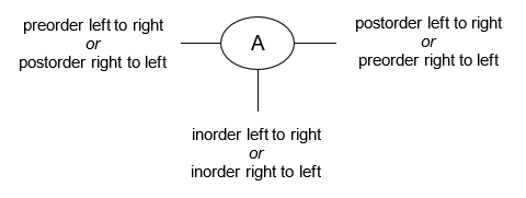
The point at which the path you've drawn around the binary tree intersects the tick mark is the point at which that node will be "visited" during the traversal. Examples for pre-, post-, and in-order traversals are provided below (left-to-right and right-to-left).
Why the tick trick actually works
The "tick trick" is a very nice, effective way to get a quick handle on the order in which nodes of a tree will be traversed. But why does drawing the tick in the manner specified actually work in creating the effective visual?
Perhaps the first key observation to keep in mind is how we actually start drawing any path that is meant to represent a traversal, namely not only from the root but from above whatever edges connect the root to other nodes; that is, we do not trace out a path from the root by drawing from the bottom of the node (no matter what kind of traversal we are doing). We start tracing the path above the edge that connects the root to its left child (or right child if we are doing a reverse traversal). Effectively, we start tracing out the path by starting from the top of the root node and then going the desired direction (conventionally left). These may seem like minor observations, but they are important to specify in order to make our path drawings well-defined (otherwise the "tick trick" could have different meanings for different path drawings).
Drawing a path around the tree, in the manner specified above, and placing tick marks at strategic points on the nodes allows us to create a visual guide that effectively conveys the sequence of node visits, where a "visit" represents the processing of a node and is visually indicated by the path intersecting the tick drawn on the node:
-
Pre-order: The idea is to draw the tick on the node in such a way that we cannot visit any of the node's children (left or right) before visiting the node itself. We can do this by drawing the tick on the left side of the node. The path traced out must intersect the node's tick before proceeding down the tree (i.e., before visiting any children).
Recursive observation: The practical implication of this tracing/traversal is that, starting at
node(regardless of reference point), we processnodeand its entire left subtree before moving on to process nodes in the right subtree ofnode. We travel as deeply as we can to the left, processing each node as we encounter it. Only once we've fully exhausted our abilities to go left do we start to go right by means of backtracking (this is indicated in the path tracing by the tracing moving upward and then back down to cover the right subtree). -
In-order: How can we draw the tick in such a way that makes it clear the current node cannot be visited until
- after its left child has been visited and
- before its right child has been visited?
The way in which we are tracing out a path suggests a possibility (think of a tree rooted at
1with left child2and right child3): if we draw the tick straight down from the node, then we can only intersect the tick of the current node after intersecting the tick of its left child; furthermore, as we start to backtrack to visit the right child, we must cross the tick of the current node before reaching its right child.Recursive observation: The practical implication of this tracing/traversal is that, starting at
node(regardless of reference point), we processnodeonly after its entire left subtree has been processed and before its right subtree. This is why in-order traversal is common for binary search trees (BST), where the node values are ordered in a certain way: in-order traversal from left to right ensures nodes are processed in ascending order according to their value; similarly, in-order traversal of a BST from right-to-left ensures nodes are processed in descending order according to their value. -
Post-order: How can we draw the tick in such a way that makes it clear a node is only visited once its children have been visited? Directionally, it seems like a node's tick should be intersected by the path tracing once the path has gone as deep as it can (i.e., visited its children) and it is time to go back up and away. We can accomplish this by drawing the tick on the right side of a node, where the path is leaving the node in an upward direction.
Recursive observation: The practical implication of this tracing/traversal is that, starting at
node(regardless of reference point), we processnodeonly after its entire left subtree and its entire right subtree have been processed.
Correspondence between left-to-right and right-to-left traversals
It may be tempting to think that right-to-left traversals should effectively be "reversals" of their left-to-right counterparts, but this is not the case for pre- and post-order traversals. It is only the case for in-order traversals.
To see why, recall what the various traversals actually mean. A pre-order traversal means we will visit the current node before traversing either of its subtrees whereas a post-order traversal means we will visit the current node after traversing both of its subtrees. In either case, the root node itself serves as a point of clarification:
__A______ | Pre-order (L -> R): A B X E M S W T P N C H
/ \ | Pre-order (R -> L): A W C H T N P B S X M E
__B __W__ | Post-order (L -> R): E M X S B P N T H C W A
/ \ / \ | Post-order (R -> L): H C N P T W S M E X B A
X S T C | In-order (L -> R): E X M B S A P T N W H C
/ \ / \ / | In-order (R -> L): C H W N T P A S B M X E
E M P N H |
How could the left-to-right and right-to-left pre-order traversals be reversals of each other if they both start with the same node? Similarly, the post-order traversals cannot be reversals of each other if they both end with the same node. But what about in-order traversals? As can be seen above, the order in which the nodes are visited is reversed when we change the traversal from left-to-right to right-to-left.
It is worth noting that the left-to-right pre-order traversal is effectively the reverse of the right-to-left post-order traversal. Similarly, the left-to-right post-order traversal is effectively the reverse of the right-to-left pre-order traversal.
Use the binarytree package in Python to facilitate learning
Learning about trees can become overly cumbersome if you are specifying all of the nodes yourself. For example, the binary tree in the tip above (and the one we will see throughout the subsections below) may be set up in Python without any package support as follows:
See the setup
class TreeNode:
def __init__(self, val, left=None, right=None):
self.val = val
self.left = left
self.right = right
n1 = TreeNode('A')
n2 = TreeNode('B')
n3 = TreeNode('W')
n4 = TreeNode('X')
n5 = TreeNode('S')
n6 = TreeNode('T')
n7 = TreeNode('C')
n8 = TreeNode('E')
n9 = TreeNode('M')
n10 = TreeNode('P')
n11 = TreeNode('N')
n12 = TreeNode('H')
n1.left = n2
n1.right = n3
n2.left = n4
n2.right = n5
n4.left = n8
n4.right = n9
n3.left = n6
n3.right = n7
n6.left = n10
n6.right = n11
n7.left = n12
That's not fun. The binarytree package makes things much easier to work with. The same tree can be set up as follows:
from binarytree import build2
bin_tree = build2(['A', 'B', 'W', 'X', 'S', 'T', 'C', 'E', 'M', None, None, 'P', 'N', 'H'])
The code in the sections below will rely on binarytree for the sake of simplicity.
- Pre-order (L->R)
- Pre-order (R->L)
- Post-order (L->R)
- Post-order (R->L)
- In-order (L->R)
- In-order (R->L)
- Level-order (L->R)
- Level-order (R->L)

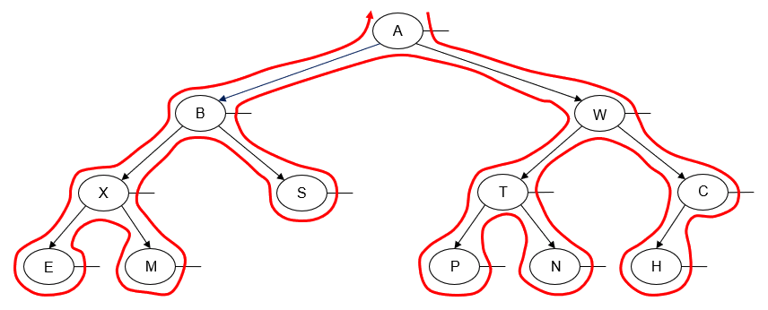
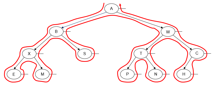
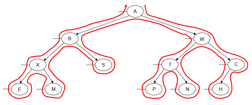
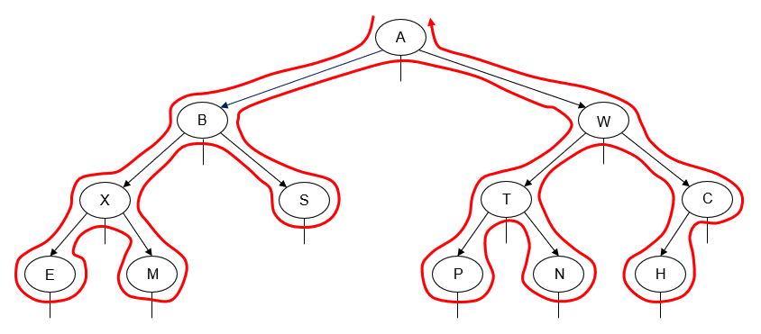
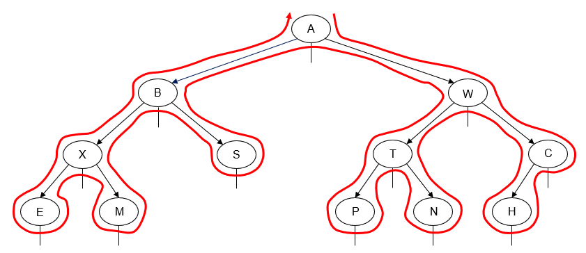
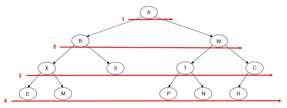
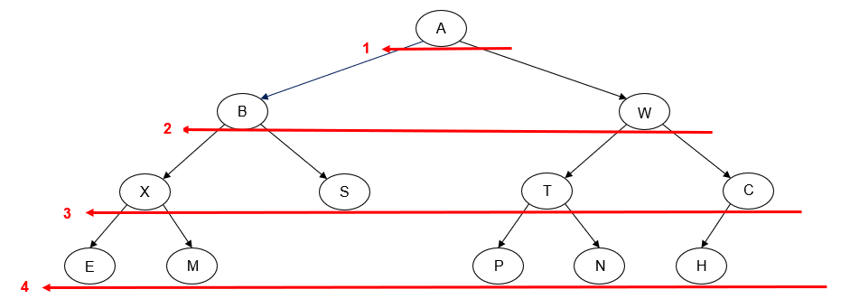
Pre-order traversal
Recursive
Remarks
TBD
- Python (L->R)
- Python (R->L)
- Pseudocode
def preorder_recursive_LR(node):
if not node:
return
visit(node)
preorder_recursive_LR(node.left)
preorder_recursive_LR(node.right)
def preorder_recursive_RL(node):
if not node:
return
visit(node)
preorder_recursive_RL(node.right)
preorder_recursive_RL(node.left)
procedure preorder(node)
if node = null
return
visit(node)
preorder(node.left)
preorder(node.right)
Examples
TBD
Iterative
Remarks
TBD
Analogy
procedure iterativePreorder(node)
if node = null
return
stack ← empty stack
stack.push(node)
while not stack.isEmpty()
node ← stack.pop()
visit(node)
if node.right ≠ null
stack.push(node.right)
if node.left ≠ null
stack.push(node.left)
Imagine you're a tourist visiting a town rapidly growing in popularity. This town has several attractions, and you want to start by seeing the the main one (root). In an effort to help tourists plan their sightseeing effectively, town leadership organized the attractions in such a way that subsequent attractions are usually recommended once a tourist has finished visiting the current attraction. Any given attraction will recommend either no subsequent attraction (a leaf), a single subsequent attraction, or two subsequent attractions. If two subsequent attractions are recommended, then one will be a primary attraction (left child) and the other a secondary attraction (right child). You want to see as many primary attractions as you can, starting at the main primary attraction, before moving on to secondary attractions, but you want to see them all.
Here's the process you will follow in order to accomplish this:
- Step 1 (start seeing attractions): Begin your sightseeing journey by visiting the town's main attraction (visit the root).
- Step 2 (note the recommendations): If the attraction you just visited recommends another attraction (not a leaf), then make a note of this (push to the stack).
- Step 3 (visit primary attractions first and as encountered): Before exploring the town any further and visiting other attractions, always immediately visit the recommended primary attraction (left child) if it exists.
- Step 4 (note secondary attractions): If the attraction you just visited recommends a secondary attraction (right child), then note this secondary attraction for visiting later (push to the stack), but continue on your current path.
- Step 5 (use your notes to visit more attractions): Once you have finished seeing as many consecutive primary attractions as you can, consult your notes and follow your most recent note about secondary attractions that you've made.
- Step 6 (finish seeing attractions): Continue the pattern of visiting primary attractions as you encounter them and noting down secondary attractions for future visitations until you have explored all attractions in the town.
We can annotate the previously provided Python code to illustrate the steps above (the highlighted line simply serves to show where the logic would be included to process the current node):
def preorder_iterative_LR(node):
# (in case there is no main attraction)
if not node:
return
stack = []
stack.append(node) # Step 1: Start seeing attractions
while stack:
node = stack.pop() # Step 3 or 5: Visit primary attraction (Step 3) OR
# check most recent note for secondary attraction (Step 5)
visit(node) # Visit the current attraction (process current node)
# Step 4: Note the recommended secondary attraction (if it exists)
if node.right:
stack.append(node.right)
# Step 2: Note the recommended primary attraction (if it exists)
if node.left:
stack.append(node.left)
Note that since stacks are fundamentally LIFO structures (i.e., last in first out) we want to push primary attraction recommendations to the stack after secondary attraction recommendations. This ensures we always get the primary attraction recommendation when we pop from the stack.
This analogy makes it clear the tourist focuses on the primary attractions but neither loses sight of nor forgets the secondary attractions thanks to the notes taken after visiting each attraction (i.e., pushing to the stack).
- Python (L->R)
- Python (R->L)
- Pseudocode
def preorder_iterative_LR(node):
if not node:
return
stack = []
stack.append(node)
while stack:
node = stack.pop()
visit(node)
if node.right:
stack.append(node.right)
if node.left:
stack.append(node.left)
def preorder_iterative_RL(node):
if not node:
return
stack = []
stack.append(node)
while stack:
node = stack.pop()
visit(node)
if node.left:
stack.append(node.left)
if node.right:
stack.append(node.right)
procedure iterativePreorder(node)
if node = null
return
stack ← empty stack
stack.push(node)
while not stack.isEmpty()
node ← stack.pop()
visit(node)
// right child is pushed first so that left is processed first
if node.right ≠ null
stack.push(node.right)
if node.left ≠ null
stack.push(node.left)
Examples
TBD
Post-order traversal
Recursive
Remarks
TBD
- Python (L->R)
- Python (R->L)
- Pseudocode
def postorder_recursive_LR(node):
if not node:
return
postorder_recursive_LR(node.left)
postorder_recursive_LR(node.right)
visit(node)
def postorder_recursive_RL(node):
if not node:
return
postorder_recursive_RL(node.right)
postorder_recursive_RL(node.left)
visit(node)
procedure postorder(node)
if node = null
return
postorder(node.left)
postorder(node.right)
visit(node)
Examples
TBD
Iterative
Remarks
TBD
Analogy
procedure iterativePostorder(node)
stack ← empty stack
lastNodeVisited ← null
while not stack.isEmpty() or node ≠ null
if node ≠ null
stack.push(node)
node ← node.left
else
peekNode ← stack.peek()
if peekNode.right ≠ null and lastNodeVisited ≠ peekNode.right
node ← peekNode.right
else
visit(peekNode)
lastNodeVisited ← stack.pop()
def postorder_iterative_LR(node):
stack = []
last_node_visited = None
while stack or node:
if node:
stack.append(node)
node = node.left
else:
peek_node = stack[-1]
if peek_node.right and (last_node_visited is not peek_node.right):
node = peek_node.right
else:
visit(peek_node)
last_node_visited = stack.pop()
Imagine you're exploring a series of underground caves, where the caves have multiple tunnels (paths) and chambers (nodes) connected in a complex network. Your ultimate goal is to mark each chamber as having been "Explored", but you can only mark a chamber as having been "Explored" if you have explored all the deeper chambers (children) accessible from it. To accomplish this task, you have been given a piece of chalk for marking chambers and a map to record where you have been. Every time you enter a new chamber, you mark it on your map (push it to the stack), but you hold off on marking the chamber as "Explored" until you've visited every chamber accessible from it.
Here's the process you will follow in order to accomplish this:
- Step 1 (begin the exploration): Enter the first chamber (root).
- Step 2 (check for a left tunnel): Check for a left tunnel. If there is a left tunnel, then mark this chamber on your map (push to the stack) and venture down the left tunnel.
- Step 3 (exhaust all left tunnels): Continue to the deepest chamber you can reach by always taking left tunnels.
- Step 4 (check for a right tunnel): Check for a right tunnel once you find yourself in a chamber with no left tunnel or where all left chambers have been marked as "Explored".
- Step 5 (venture down a right tunnel): If there's an unexplored right tunnel, mark your current chamber on the map (it's still on the stack) and venture down the right tunnel.
- Step 6 (mark a chamber as "Explored"): If there's no right tunnel or if it's already been explored, then this chamber is now the deepest unexplored one, so you can mark it as "Explored" (visit the node by printing its value). Then cross it off your map (pop it from the stack) and backtrack.
- Step 7 (continue the process): Continue the process described above. Every time you backtrack to a chamber, check its right tunnel. If it's unexplored, then venture in. If it's explored or non-existent, then mark the chamber as "Explored" and backtrack further.
- Step 8 (return to the entrance): Keep doing everything above until you've marked every chamber as "Explored" and have returned to the cave entrance.
Essentially, you will be venturing down as deep as you can, marking chambers as "Explored" on your way out, ensuring the deeper chambers are always marked as "Explored" before the shallower ones from which they are accessible.
We can annotate the previously provided Python code to illustrate the steps above (the highlighted line simply serves to show where the logic would be included to process the current node):
def postorder_iterative_LR(node):
stack = []
last_node_visited = None
# Step 1: Enter the cave system. As long as there's a chamber to explore
# or a path in the stack to backtrack to, continue.
while stack or node:
# Step 2: If you're in a new chamber, then mark the path you took
# to get there (push it onto a stack).
if node:
stack.append(node)
# Step 3: Always check the left tunnel of the current chamber first.
# If there is one, you go down it.
node = node.left
else:
# Step 4: If there's no left tunnel or after coming back
# from a left tunnel, you're ready to check the right tunnel.
peek_node = stack[-1]
# Step 5: Before checking the right tunnel,
# make sure you haven't just explored it.
# If not, you go down the right tunnel.
if peek_node.right and (last_node_visited is not peek_node.right):
node = peek_node.right
else:
# Step 6: If no tunnels remain to explore from current chamber,
# or if you've just explored the right tunnel, then
# it's time to mark the current chamber as "Explored"
visit(peek_node)
# Step 7: After marking the chamber as "Explored", you backtrack.
# The last path you took (from the stack) will help you go back.
last_node_visited = stack.pop()
# Step 8: When you've explored every chamber and every tunnel,
# and there's no path left in your stack,
# you exit the cave system.
It's worth specifically noting what the following if block accomplishes in the code above:
if peek_node.right and (last_node_visited is not peek_node.right):
node = peek_node.right
peek_node.right: This checks whether or nor the current chamber (represented bypeek_node) has a right tunnel and answers the question, "Is there a right tunnel leading out of this chamber?"last_node_visited is not peek_node.right: This checks if the right tunnel/chamber (peek_node.right) was the last one you explored. If it was, then you've already visited it and don't need to venture down there again. It answers the question, "Did I just come from that right tunnel, or have I not explored it yet?"node = peek_node.right: If the current chamber has an unexplored right tunnel, then prepare to venture into it. This assignment is effectively saying, "I haven't explored the right tunnel of this chamber yet. Let's go down there next."
Essentially, the if block above ensures you explore a chamber's right tunnel if you haven't already — if you've just come back from exploring the right tunnel (i.e., last_node_visited is peek_node.right is True), then you know it's time to mark the current chamber as "Explored" and backtrack.
The procedure outlined above is rather sophisticated and complex in its logic — it is probably easiest to understand if we actually work through a concrete example such as the one provided below (writing out the process may seem tedious, and it is, but it's worth following the first time around to provide some sort of intuition for things).
Concrete example using a familiar binary tree
We have used the following binary tree in a number of previous examples:
__A______
/ \
__B __W__
/ \ / \
X S T C
/ \ / \ /
E M P N H
For the sake of our example, suppose each node represents a chamber of a cave. Then the entrance to the cave system is marked by the root node, A. Let's start exploring the cave and try to mark all chambers as "Explored" by using our previously described process, where the order in which the chambers should be marked as "Explored" should be E M X S B P N T H C W A in order to hold true to a post-order traversal (each bullet point below represents an iteration of the while loop where each bullet point ends with the current state of explored chambers):
-
We start by entering the cave system, leading us into chamber
A. We push this on to the stack:| A |
+---+We attempt to go to chamber
A's left tunnel if there is one. There is. We update the current node to point to chamberB.Explored chambers:
[] -
We push
Bon to the stack:| B |
| A |
+---+We attempt to go to chamber
B's left tunnel if there is one. There is. We update the current node to point to chamberX.Explored chambers:
[] -
We push
Xon to the stack:| X |
| B |
| A |
+---+We attempt to go to chamber
X's left tunnel if there is one. There is. We update the current node to point to chamberE.Explored chambers:
[] -
We push
Eon to the stack:| E |
| X |
| B |
| A |
+---+We attempt to go to chamber
E's left tunnel if there is one. There is not. We update the current node to point toNone.Explored chambers:
[] -
Since
nodecurrently points toNone, we do not need to check for a left tunnel. Instead, we need to check for a right tunnel.peek_node = stack[-1]meanspeek_nodepoints to nodeEsinceEis on top of the stack.peek_node.righthas no meaningful value since chamberEhas no right tunnel; hence, no tunnels remain to explore from our current chamber. We can mark chamberEas "Explored". To keep track of which chamber we last visited and to update our stack of chambers we still need to explore, we letlast_node_visited = stack.pop(), meaninglast_node_visitednow points to nodeE, and our updated stack looks as follows:| X |
| B |
| A |
+---+Explored chambers:
[ E ] -
Since
nodestill points toNone, we do not need to check for a left tunnel. Instead, we need to check for a right tunnel.Simplify Matters by Understanding the Possible Outcomes for Each IterationIt is easy to get lost in some of the fancy referential footwork used in the iterative post-order traversal. But note the only possible outcomes for each iteration of the
whileloop:-
(left tunnel exists): enter chamber of left tunnel and keep going left until you can go no further
-
(no left tunnel; no right tunnel): mark the chamber as explored (print the node's value), note the chamber as being the last one explored, and remove the chamber from the stack of chambers waiting to be explored
-
(no left tunnel; right tunnel exists, not yet explored): enter chamber of right tunnel and try to explore its left tunnels if it has any
-
(no left tunnel; right tunnel exists, already explored): this is effectively the same as neither having a left tunnel nor a right tunnel — follow the guidelines above concerning that scenario
Essentially, you're going left or right if you can; otherwise, you're marking the chamber as having been explored (printing its value), noting that you just explored it so you don't explore it again and updating the stack of chambers that need exploring (popping from the stack the chamber you just visited and referring to it as
last_node_visited).Since
Xnow sits at the top of the stack,peek_node = stack[-1]meanspeek_nodepoints to chamberX. This timepeek_node.rightdoes have a meaningful value since there is a right tunnel from chamberXthat leads into chamberM. Before we visit chamberM, however, we need to ask ourselves, "Have we visited chamberMyet?" Sincelast_node_visitedpoints to chamberEand not chamberM, we can safely assume we have not yet visited chamberM. As such, we should prepared to visit chamberM. Updatenodeto point to chamberM.Explored chambers:
[ E ] -
-
We push
Mon to the stack:| M |
| X |
| B |
| A |
+---+We attempt to go to chamber
M's left tunnel if there is one. There is not. We update the current node to point toNone.Explored chambers:
[ E ] -
peek_node = stack[-1]now points to chamberM. There's no right tunnel from chamberM. Mark chamberMas having been explored, and pop it from the stack of chambers we still need to visit (make sure to keep a reference to this most recently explored chamber as well):| X |
| B |
| A |
+---+Explored chambers:
[ E M ] -
Since
nodestill points toNone, we look at chamberpeek_node = stack[-1], which points again to chamberX. Note thatpeek_node.rightgives a meaningful value, namely chamberM. But we just visited chamberMand marked it as explored. Visiting chamberMagain would not make any sense. Fortunately, we noted which chamber we last visited withlast_node_visited. This variable points to chamberM.Hence, the second part of the
andportion ofpeek_node.right and (last_node_visited is not peek_node.right)is false, meaning we do not explore the right tunnel (i.e., chamber
M). This means we can now safely mark chamberXas having been explored (since all chambers beneath it on the left and right have now been explored) as well as update our stack and our "most recently visited chamber" reference:| B |
| A |
+---+Explored chambers:
[ E M X ] -
The pattern may start to emerge more clearly now.
nodestill points toNone.peek_node = stack[-1]meanspeek_nodenow points to chamberB. We see thatpeek_node.righthas a meaningful value, namely chamberS. Furthermore,last_node_visitedpoints to chamberX, not chamberS. Hence, we should explore the right tunnel from chamberBthat begins with chamberS.Explored chambers:
[ E M X ] -
nodenow points to chamberS. Push it to the stack:| S |
| B |
| A |
+---+We attempt to go to chamber
S's left tunnel if there is one. There is not. We update the current node to point toNone.Explored chambers:
[ E M X ] -
nodenow points toNone. Andpeek_node = stack[-1]points to chamberS. Andpeek_node.rightdoes not give a meaningful value, meaning chamberShas no right tunnel. Mark chamberSas explored and pop it from the stack:| B |
| A |
+---+Update our reference for the most recently explored chamber.
Explored chambers:
[ E M X S ] -
nodepoints toNone.peek_node = stack[-1]points to chamberBagain.peek_node.rightpoints to chamberS, butlast_node_visitedalso points to chamberS. Hence, mark chamberBas explored and pop it from the stack:| A |
+---+Update our reference for the most recently explored chamber.
Explored chambers:
[ E M X S B ] -
nodepoints toNone.peek_node = stack[-1]points to chamberA.peek_node.rightpoints to chamberW. Sincelast_node_visitedpoints to chamberBand not chamberW, this means we should prepare to visit the right tunnel from chamberAthat begins with chamberW. Updatenodeto point to chamberW.Explored chambers:
[ E M X S B ] -
nodepoints to chamberW. Push it to the stack:| W |
| A |
+---+We attempt to go to chamber
W's left tunnel if there is one. There is. We update the current node to point to chamberT.Explored chambers:
[ E M X S B ] -
nodepoints to chamberT. Push it to the stack:| T |
| W |
| A |
+---+We attempt to go to chamber
T's left tunnel if there is one. There is. We update the current node to point to chamberP.Explored chambers:
[ E M X S B ] -
nodepoints to chamberP. Push it to the stack:| P |
| T |
| W |
| A |
+---+We attempt to go to chamber
P's left tunnel if there is one. There is not. We update the current node to point toNone.Explored chambers:
[ E M X S B ] -
nodepoints toNone. Andpeek_node = stack[-1]points to chamberP. Sincepeek_node.rightdoes not have a meaningful value (i.e., chamberPhas no right tunnel), we may mark chamberPas explored and pop it from the stack:| T |
| W |
| A |
+---+Update our reference for the most recently explored chamber.
Explored chambers:
[ E M X S B P ] -
nodepoints toNone. Andpeek_node = stack[-1]points to chamberT. We look for a right tunnel and see thatpeek_node.rightreveals chamberN. Sincelast_node_visitedpoints to chamberPand not chamberN, we prepare to explore chamberN. Updatenodeto point to chamberN.Explored chambers:
[ E M X S B P ] -
nodepoints to chamberN. Push it to the stack:| N |
| T |
| W |
| A |
+---+We attempt to go to chamber
N's left tunnel if there is one. There is not. We update the current node to point toNone.Explored chambers:
[ E M X S B P ] -
nodepoints toNone. Andpeek_node = stack[-1]points to chamberN. Sincepeek_node.rightdoes not provide a meaningful value (i.e., chamberNhas no right tunnel), we may mark chamberNas explored and pop it from the stack:| T |
| W |
| A |
+---+Update our reference for the most recently explored chamber.
Explored chambers:
[ E M X S B P N ] -
nodepoints toNone. Andpeek_node = stack[-1]points to chamberTagain. Andpeek_node.rightpoints to chamberN. Butlast_node_visitedalso points to chamberN, indicating we should not explore chamberN. Instead, we should mark chamberTas explored and pop it from the stack:| W |
| A |
+---+Update our reference for the most recently explored chamber.
Explored chambers:
[ E M X S B P N T ] -
nodepoints toNone. Andpeek_node = stack[-1]points to chamberW. Andpeek_node.rightpoints to chamberC. Sincelast_node_visitedpoints to chamberTand not chamberC, we should prepare to visit chamberC. Updatenodeto point to chamberC.Explored chambers:
[ E M X S B P N T ] -
nodepoints to chamberC. Push it to the stack:| C |
| W |
| A |
+---+We attempt to go to chamber
C's left tunnel if there is one. There is. We update the current node to point to chamberH.Explored chambers:
[ E M X S B P N T ] -
nodepoints to chamberH. Push it to the stack:| H |
| C |
| W |
| A |
+---+We attempt to go to chamber
H's left tunnel if there is one. There is not. We update the current node to point toNone.Explored chambers:
[ E M X S B P N T ] -
nodepoints toNone. Andpeek_node = stack[-1]points to chamberH. Sincepeek_node.rightdoes not provide a meaningful value, we may mark chamberHas being explored and pop it from the stack:| C |
| W |
| A |
+---+Update our reference for the most recently explored chamber.
Explored chambers:
[ E M X S B P N T H ] -
nodepoints toNone. Andpeek_node = stack[-1]points to chamberC. Sincepeek_node.rightdoes not provide a meaningful value, we may mark chamberCas explored and pop it from the stack:| W |
| A |
+---+Update our reference for the most recently explored chamber.
Explored chambers:
[ E M X S B P N T H C ] -
nodepoints toNone. Andpeek_node = stack[-1]points to chamberW. Even thoughpeek_node.rightpoints to chamberC, we see thatlast_node_visitedalso points to chamberC, meaning we should not visit chamberC. Mark chamberWas explored and pop it from the stack:| A |
+---+Update our reference for the most recently explored chamber.
Explored chambers:
[ E M X S B P N T H C W ] -
nodepoints toNone. Andpeek_node = stack[-1]points to chamberA. Even thoughpeek_node.rightpoints to chamberW, we see thatlast_node_visitedalso points to chamberW, meaning we should not visit chamberW. Mark chamberAas explored and pop it from the stack:[]Update our reference for the most recently explored chamber.
Explored chambers:
[ E M X S B P N T H C W A ]
The while loop does not fire now since node still points to None and stack is now empty. The iterative post-order traversal is now complete, and we see we have visited the chambers in the expected order:
E M X S B P N T H C W A
In sum, iterative post-order traversals can be rather complicated, but can also be elegant nonetheless.
- Python (L->R)
- Python (R->L)
- Pseudocode
def postorder_iterative_LR(node):
stack = []
last_node_visited = None
while stack or node:
if node:
stack.append(node)
node = node.left
else:
peek_node = stack[-1]
if peek_node.right and (last_node_visited is not peek_node.right):
node = peek_node.right
else:
visit(peek_node)
last_node_visited = stack.pop()
def postorder_iterative_RL(node):
stack = []
last_node_visited = None
while stack or node:
if node:
stack.append(node)
node = node.right
else:
peek_node = stack[-1]
if peek_node.left and (last_node_visited is not peek_node.left):
node = peek_node.left
else:
visit(peek_node)
last_node_visited = stack.pop()
procedure iterativePostorder(node)
stack ← empty stack
lastNodeVisited ← null
while not stack.isEmpty() or node ≠ null
if node ≠ null
stack.push(node)
node ← node.left
else
peekNode ← stack.peek()
// if right child exists and traversing node
// from left child, then move right
if peekNode.right ≠ null and lastNodeVisited ≠ peekNode.right
node ← peekNode.right
else
visit(peekNode)
lastNodeVisited ← stack.pop()
Examples
TBD
In-order traversal
Recursive
Remarks
TBD
- Python (L->R)
- Python (R->L)
- Pseudocode
def inorder_recursive_LR(node):
if not node:
return
inorder_recursive_LR(node.left)
visit(node)
inorder_recursive_LR(node.right)
def inorder_recursive_RL(node):
if not node:
return
inorder_recursive_RL(node.right)
visit(node)
inorder_recursive_RL(node.left)
procedure inorder(node)
if node = null
return
inorder(node.left)
visit(node)
inorder(node.right)
Examples
TBD
Iterative
Remarks
TBD
Analogy
procedure iterativeInorder(node)
stack ← empty stack
while not stack.isEmpty() or node ≠ null
if node ≠ null
stack.push(node)
node ← node.left
else
node ← stack.pop()
visit(node)
node ← node.right
Imagine you're reading a book series. Specifically, let's suppose you're reading the Jack Ryan series of novels by Tom Clancy. You've heard a lot about this series and know several books have film adaptations. You'd like to check it out. The first book you check out, Debt of Honor, seems to probably end with Jack Ryan becoming the President of the United States. That can't be right. Surely there's a lot more to Jack Ryan's story that led up to that point. You'd really like to read the whole book series in order, specifically by chronological order of events as opposed to publication date.
Jack Ryan novels by chronological order of events
The excerpt below is from ChatGPT (Aug 19, 2023).
Tom Clancy's Jack Ryan series, with its complex web of interconnected characters and plots, can be arranged according to the internal chronological order of events rather than their publication dates. This order provides a coherent understanding of Jack Ryan's life, from a young Marine to President of the United States, as well as the lives of other recurring characters.
Here's the chronological ordering of the Jack Ryan series based on character development and the events in the series:
-
Without Remorse (1993) - This novel serves as a prequel to the series, focusing on the backstory of John Kelly (who later becomes John Clark), a recurring character in many of the Jack Ryan books.
-
Red Rabbit (2002) - Set in the early 1980s, this book details a younger Jack Ryan's time with the CIA and a plot to assassinate Pope John Paul II.
-
The Hunt for Red October (1984) - This is the first novel published in the series, introducing Jack Ryan as an analyst for the CIA as he gets involved in the defection of a Soviet submarine captain.
-
The Cardinal of the Kremlin (1988) - Jack Ryan becomes involved in a high-stakes espionage game as the Americans and the Soviets vie for technological dominance.
-
Clear and Present Danger (1989) - Jack Ryan is a National Security Advisor here, and the story revolves around U.S. efforts against Colombian drug cartels.
-
The Sum of All Fears (1991) - Jack Ryan, now Deputy Director of Intelligence for the CIA, must prevent a nuclear conflict between the U.S. and Russia.
-
Debt of Honor (1994) - The focus shifts to the Pacific, with an escalating conflict between the U.S. and Japan. By the end of the novel, Jack Ryan is thrust into the role of President of the United States.
-
Executive Orders (1996) - Continuing directly from where "Debt of Honor" left off, President Ryan faces both internal and external challenges, including rebuilding the U.S. government and dealing with an Ebola-like epidemic.
-
The Bear and the Dragon (2000) - President Jack Ryan oversees a complex geopolitical situation involving China, Russia, and the prospect of World War III.
-
Red Storm Rising (1986) - While not strictly a Jack Ryan novel (he doesn't appear in it), this book is set in the same universe and involves a war between NATO and Warsaw Pact forces.
-
The Teeth of the Tiger (2003), Dead or Alive (2010), Locked On (2011), Threat Vector (2012), and Command Authority (2013) - These novels follow the next generation, including Jack Ryan Jr., as they face modern threats in a post-9/11 world. Jack Ryan Sr. still plays a role, but the torch is being passed to the younger characters.
It's worth noting that Tom Clancy's name has been attached to books written by other authors after his death in 2013. If you're interested in the books in this universe that continue the story or explore other side characters, there's an extended series to dive into, but the above list covers the main Jack Ryan saga as written by Clancy himself.
As fate would have it, the book you just started with (the root) has both prequel and sequel recommendations. Some books you encounter may have no recommendations (leaf nodes), but you want to prioritize tracing back through each preqel recommendation (left child) so you can start at the beginning of the series, but you also need to try to read the sequel (right child) for each book, as recommended.
Here's the process you will follow in order to accomplish this:
- Step 1 (start with the first book in the series): Follow all prequel recommendations (left children) from your starting point (root) until they have all been exhausted (you hit a leaf node), noting each book along the way that recommends a prequel (push it to the stack).
- Step 2 (follow recommendations): If your current book has a prequel recommendation (left child), then set it aside to be read later (push it to the stack).
- Step 3 (keep following recommendations): If the new book also has a prequel recommendation, then repeat the process: set the new book aside to read later, and pick up the recommended prequel. Continue this process until you reach a book with no prequel recommendation.
- Step 4 (read the book): Once there is no prequel left to read, read the book (visit the node).
- Step 5 (move to sequel recommendation or return to books previously set aside): Always attempt to move on to a sequel recommendation (right child) after having read a book (once the node has been visited). If there is no such sequel recommendation, then move back to the most recent book you've set aside but have not yet read (pop from the stack). Continue.
- Step 6 (repeat until all books are read): Repeat the steps above until you have finished all books in the series.
We can annotate the previously provided Python code to illustrate the steps above (the highlighted line simply serves to show where the logic would be included to process the current node):
def inorder_iterative_LR(node):
stack = []
# there is still a book to be read
while stack or node:
# Steps 1-3: Follow prequel recommendations
if node:
stack.append(node) # Step 2: Set aside the current book
node = node.left
else:
# Step 4: Read the current book
node = stack.pop()
print(node.val)
# Step 5: Move to sequel recommendation
node = node.right
Note that this analogy involves a highly contrived example. If we followed the numbering of the Jack Ryan books in chronological ordering after starting with book 7 as the root, then the most sensible binary tree would look rather ridiculous:
7
/ \
6 8
/ \
5 9
/ \
4 10
/ \
3 11
/
2
/
1
But technically any other ordering would work so long as 7 was the root and the in-order traversal led to books 1 through 11 being listed in sequence. One such example:
__7__
/ \
__5 9
/ \ / \
3 6 8 10
/ \ \
2 4 11
/
1
- Python (L->R)
- Python (R->L)
- Pseudocode
def inorder_iterative_LR(node):
stack = []
while stack or node:
if node:
stack.append(node)
node = node.left
else:
node = stack.pop()
visit(node)
node = node.right
def inorder_iterative_RL(node):
stack = []
while stack or node:
if node:
stack.append(node)
node = node.right
else:
node = stack.pop()
visit(node)
node = node.left
procedure iterativeInorder(node)
stack ← empty stack
while not stack.isEmpty() or node ≠ null
if node ≠ null
stack.push(node)
node ← node.left
else
node ← stack.pop()
visit(node)
node ← node.right
Examples
TBD
Level-order traversal
Remarks
TBD
- Python (L->R)
- Python (R->L)
- Pseudocode
- Recursive
def levelorder_LR(node):
queue = deque()
queue.append(node)
while queue:
num_nodes_this_level = len(queue)
for _ in range(num_nodes_this_level):
node = queue.popleft()
visit(node)
if node.left:
queue.append(node.left)
if node.right:
queue.append(node.right)
def levelorder_RL(node):
queue = deque()
queue.append(node)
while queue:
num_nodes_this_level = len(queue)
for _ in range(num_nodes_this_level):
node = queue.popleft()
visit(node)
if node.right:
queue.append(node.right)
if node.left:
queue.append(node.left)
procedure levelorder(node)
queue ← empty queue
queue.enqueue(node)
while not queue.isEmpty()
node ← queue.dequeue()
visit(node)
if node.left ≠ null
queue.enqueue(node.left)
if node.right ≠ null
queue.enqueue(node.right)
The pseudocode above (from Wikipedia) is the standard BFS implementation for a binary tree traversal, where we only care about visiting all nodes, level by level, left to right. But it's fairly common to encounter algorithm problems that demand you do something (i.e., perform some logic) on a level by level basis; that is, you effectively need to isolate the nodes by level. The pseudocode above does not do this, but we can easily fix this ourselves:
procedure levelorder(node)
queue ← empty queue
queue.enqueue(node)
while not queue.isEmpty()
// retrieve number of nodes on current level
numNodesThisLevel ← queue.length
// perform logic for current level
for each node in level do
node ← queue.dequeue()
// perform logic on current node
visit(node)
// enqueue nodes on next level (left to right)
if node.left ≠ null
queue.enqueue(node.left)
if node.right ≠ null
queue.enqueue(node.right)
The Python code snippets in the other tabs reflect this approach since it is the most likely approach needed in the context of solving interview problems.
As this Stack Overflow post explores, breadth-first search can be done recursively, but this does not mean it should be done recursively. It's quite a bit more complex than the iterative solution with basically no added benefit (instead of using a queue to explicitly do things efficiently we would now just be implicitly using the call stack).
That said, here's a possible recursive approach to a level-order traversal for the binary tree we've used for reference:
from binarytree import build2
bin_tree = build2(['A', 'B', 'W', 'X', 'S', 'T', 'C', 'E', 'M', None, None, 'P', 'N', 'H'])
root = bin_tree.levelorder[0]
def level_order(root):
h = height(root)
for i in range(1, h + 1):
print_level(root, i)
def print_level(node, level):
if not node:
return
if level == 1:
print(node.val)
elif level > 1:
print_level(node.left, level - 1)
print_level(node.right, level - 1)
def height(node):
if not node:
return 0
l_height = height(node.left)
r_height = height(node.right)
return max(l_height, r_height) + 1
level_order(root) # A B W X S T C E M P N H
Examples
TBD
Level-order (BFS)
Remarks
tbd
def fn(node):
queue = deque()
queue.append(node)
while queue:
num_nodes_this_level = len(queue)
for _ in range(num_nodes_this_level):
node = queue.popleft()
visit(node)
if node.left:
queue.append(node.left)
if node.right:
queue.append(node.right)
Examples
LC 199. Binary Tree Right Side View (✓)
Given the root of a binary tree, imagine yourself standing on the right side of it, return the values of the nodes you can see ordered from top to bottom.
class Solution:
def rightSideView(self, root: Optional[TreeNode]) -> List[int]:
if not root:
return root
level_node_vals_rightmost = []
queue = deque([root])
while queue:
level_node_vals_rightmost.append(queue[-1].val)
num_nodes_this_level = len(queue)
for _ in range(num_nodes_this_level):
node = queue.popleft()
if node.left:
queue.append(node.left)
if node.right:
queue.append(node.right)
return level_node_vals_rightmost
The strategy above is fairly simple — execute a left-to-right BFS traversal and pick off the rightmost node value in the queue before expanding to the next level.
LC 515. Find Largest Value in Each Tree Row (✓)
Given the root of a binary tree, return an array of the largest value in each row of the tree (0-indexed).
class Solution:
def largestValues(self, root: Optional[TreeNode]) -> List[int]:
if not root:
return []
max_level_vals = []
queue = deque([root])
while queue:
num_nodes_this_level = len(queue)
level_max = float('-inf')
for _ in range(num_nodes_this_level):
node = queue.popleft()
level_max = max(level_max, node.val)
if node.left:
queue.append(node.left)
if node.right:
queue.append(node.right)
max_level_vals.append(level_max)
return max_level_vals
Perform a level-order traversal where we push to the answer array the maximum value of each level.
LC 1302. Deepest Leaves Sum (✓)
Given the root of a binary tree, return the sum of values of its deepest leaves.
class Solution:
def deepestLeavesSum(self, root: Optional[TreeNode]) -> int:
level_sum = 0
queue = deque([root])
while queue:
num_nodes_this_level = len(queue)
curr_level_sum = 0
for _ in range(num_nodes_this_level):
node = queue.popleft()
curr_level_sum += node.val
if node.left:
queue.append(node.left)
if node.right:
queue.append(node.right)
level_sum = curr_level_sum
return level_sum
Accumulate the sum for every single level — the last sum remaining will be the sum of all the nodes in the last level.
LC 103. Binary Tree Zigzag Level Order Traversal (✓)
Given a binary tree, return the zigzag level order traversal of its nodes' values. (ie, from left to right, then right to left for the next level and alternate between).
For example: Given binary tree [3,9,20,null,null,15,7],
3
/ \
9 20
/ \
15 7
return its zigzag level order traversal as:
[
[3],
[20,9],
[15,7]
]
class Solution:
def zigzagLevelOrder(self, root: Optional[TreeNode]) -> List[List[int]]:
if not root:
return root
LEFT_RIGHT = True
node_vals = []
queue = deque([root])
while queue:
num_nodes_this_level = len(queue)
level_node_vals = []
for _ in range(num_nodes_this_level):
node = queue.popleft()
level_node_vals.append(node.val)
if node.left:
queue.append(node.left)
if node.right:
queue.append(node.right)
if not LEFT_RIGHT:
left = 0
right = len(level_node_vals) - 1
while left < len(level_node_vals) // 2:
level_node_vals[left], level_node_vals[right] = level_node_vals[right], level_node_vals[left]
left += 1
right -= 1
node_vals.append(level_node_vals)
LEFT_RIGHT = not LEFT_RIGHT
return node_vals
There are several ways to try to solve this problem, but each approach seems to involve something somewhat unnatural:
- we could use a deque for each level's values where we append to the right or append to the left depending on the level (but most BFS problems aren't supposed to explicitly rely on using deques)
- we could treat the values accumulated for each level as a stack and pop the values from the stack into another list when a right to left order is desired (but this is expensive for time and space)
- and so on
The solution above explicitly reverses a level's node values in-place, if needed. The additional space requirement is minimal since the reversal is in-place. The additional time required is also somewhat minimal since we only iterate over half the length of a level's values (the multi-deque approach avoids this additional time cost, but the use of a deque for each level seems quite unnatural).
LC 102. Binary Tree Level Order Traversal (✓)
Given a binary tree, return the level order traversal of its nodes' values. (ie, from left to right, level by level).
For example: Given binary tree [3,9,20,null,null,15,7],
3
/ \
9 20
/ \
15 7
return its level order traversal as:
[
[3],
[9,20],
[15,7]
]
class Solution:
def levelOrder(self, root: Optional[TreeNode]) -> List[List[int]]:
if not root:
return root
levels = []
queue = deque([root])
while queue:
level_vals = []
num_nodes_this_level = len(queue)
for _ in range(num_nodes_this_level):
node = queue.popleft()
level_vals.append(node.val)
if node.left:
queue.append(node.left)
if node.right:
queue.append(node.right)
levels.append(level_vals)
return levels
Most BFS problems require some ingenuity, but this problem is mostly a basic test — the primary gotcha can occur if you don't account for a missing root properly. The rest of the solution is simply traversing level by level and pushing each level's values to level_vals before pushing level_vals to levels once the level has been entirely processed.
LC 1161. Maximum Level Sum of a Binary Tree (✓)
Given the root of a binary tree, the level of its root is 1, the level of its children is 2, and so on.
Return the smallest level x such that the sum of all the values of nodes at level x is maximal.
class Solution:
def maxLevelSum(self, root: Optional[TreeNode]) -> List[List[int]]:
max_level = 0
level = 0
max_level_sum = float('-inf')
queue = deque([root])
while queue:
level += 1
level_sum = 0
num_nodes_this_level = len(queue)
for i in range(num_nodes_this_level):
node = queue.popleft()
level_sum += node.val
if node.left:
queue.append(node.left)
if node.right:
queue.append(node.right)
if level_sum > max_level_sum:
max_level = level
max_level_sum = level_sum
return max_level
This is a fun one. Keep track of which level you are processing as well as its sum. Only update max_level and max_level_sum if the current level sum is greater than all previously encountered level sums.
LC 637. Average of Levels in Binary Tree (✓)
Given the root of a binary tree, return the average value of the nodes on each level in the form of an array. Answers within 10-5 of the actual answer will be accepted.
class Solution:
def averageOfLevels(self, root: Optional[TreeNode]) -> List[float]:
level_avgs = []
queue = deque([root])
while queue:
level_sum = 0
num_nodes_this_level = len(queue)
for _ in range(num_nodes_this_level):
node = queue.popleft()
level_sum += node.val
if node.left:
queue.append(node.left)
if node.right:
queue.append(node.right)
level_avgs.append(level_sum / num_nodes_this_level)
return level_avgs
Executing a BFS and keeping track of each level is clearly a very common pattern. Computing the level average is much easier when using this pattern.
LC 1609. Even Odd Tree (✓) ★★
A binary tree is named Even-Odd if it meets the following conditions:
- The root of the binary tree is at level index
0, its children are at level index1, their children are at level index2, etc. - For every even-indexed level, all nodes at the level have odd integer values in strictly increasing order (from left to right).
- For every odd-indexed level, all nodes at the level have even integer values in strictly decreasing order (from left to right).
Given the root of a binary tree, return true if the binary tree is Even-Odd, otherwise return false.
class Solution:
def isEvenOddTree(self, root: Optional[TreeNode]) -> bool:
queue = deque([root])
required_remainder = 1
while queue:
num_nodes_this_level = len(queue)
most_recent_val = float('-inf') if required_remainder else float('inf')
for _ in range(num_nodes_this_level):
node = queue.popleft()
if node.val % 2 != required_remainder:
return False
elif required_remainder and most_recent_val >= node.val:
return False
elif not required_remainder and most_recent_val <= node.val:
return False
most_recent_val = node.val
if node.left:
queue.append(node.left)
if node.right:
queue.append(node.right)
required_remainder = (required_remainder + 1) % 2
return True
This is a tougher BFS problem, one that is deceptively more difficult than it appears to be at first glance. The solution above relies on exploiting the truthy or falsy nature of required_remainder for a number of things, including parity checks.
Induction (solve subtrees recursively, aggregate results at root)
Remarks
Core idea: Solve the problem at the subtrees recursively, and then aggregate the results at the root.
This template is for problems where the solutions for the subtrees is enough to find the solution for the entire tree. We call it induction because we treat each node as the root of its own subtree, and each subtree has its own solution (we "forget" that there is more tree above it). However, sometimes the solutions for the subtrees are not enough to find the solution for the entire tree, so this template can be too limiting, in which case we move to the traverse-and-accumulate template.
Note: This template effectively uses a post-order traversal since the root is only being processed in the return value when root.val is reported.
Consider the problem of finding the maximum difference between any two values in a binary tree. We cannot answer this question using just the induction template. Why? Because the smallest and largest node values could reside in different subtrees (at different levels). Using the induction tempalte, there's not an effective way to manage this information.
We need something more, namely the traverse-and-accumulate method where we can traverse the entire tree, accumulating the maximum and minimum node values along the way. Our final step would be to report the difference between these values.
def solution(root):
if not root:
return ...
res_left = solution(root.left)
res_right = solution(root.right)
# return a value computed via res_left, res_right, and root.val
return ...
Examples
Number of leaves in a binary tree (not on LeetCode)
def num_leaves(root):
if not root:
return 0
if not root.left and not root.right:
return 1
left = num_leaves(root.left)
right = num_leaves(root.right)
return left + right
A non-existent node should not count anything towards the overall number of leaf nodes. Return 0 for non-existent nodes. If we encounter a leaf node, then we will return 1 in order to include that number in the overall aggregated result.
Test for value in a binary tree (not on LeetCode)
def has_value(root, target):
if not root:
return False
if root.val == target:
return True
left = has_value(root.left, target)
right = has_value(root.right, target)
return left or right
Calculate tree size (not on LeetCode)
def tree_size(root):
if not root:
return 0
left = tree_size(root.left)
right = tree_size(root.right)
return 1 + left + right
Count the total number of nodes in the tree by counting the nodes in each subtree and then add 1 for the root (this means we're always adding 1 for each node we encounter since each node encountered is treated as the root of its own subtree).
Find the maximum value in a binary tree (not on LeetCode)
def max_tree_val(root):
if not root:
return float('-inf')
left = max_tree_val(root.left)
right = max_tree_val(root.right)
return max(root.val, left, right)
This is also a situation where it's completely possible and natural, albeit unnecessary, to find the maximum by "accumulating" the result in a max_val non-local variable which we update whenever we find a new maximum value (i.e., we're basically doing a for loop through all the nodes in the tree):
def max_tree_val(root):
max_val = root.val
def visit(node):
if not node:
return float('-inf')
nonlocal max_val
max_val = max(max_val, node.val)
visit(node.left)
visit(node.right)
visit(root)
return max_val
LC 104. Maximum Depth of Binary Tree (✓)
Given the root of a binary tree, return its maximum depth.
A binary tree's maximum depth is the number of nodes along the longest path from the root node down to the farthest leaf node.
Approach 1 (no helper function, aggregated total height)
class Solution:
def maxDepth(self, root: Optional[TreeNode]) -> int:
if not root:
return 0
left = self.maxDepth(root.left)
right = self.maxDepth(root.right)
return 1 + max(left, right)
Solving the tree problem inductively means looking at the left and right children of root as roots of their own subtrees. Looking at the leaves will always be a hint as to how you should handle base cases. What should happen as soon as we hit a leaf? What is the height of a leaf node? The height should be 1 since the height of a leaf node really just includes the leaf node itself since it doesn't have any children.
The idea is to always add 1 to the height of a result in order to account for the current node — this includes leaf nodes. A leaf node's left and right non-existent children will both contribute 0 to its height: 1 + max(0, 0). That's the idea in this problem.
Approach 2 (visit helper function with accumulated max height)
class Solution:
def maxDepth(self, root: Optional[TreeNode]) -> int:
def visit(node, height):
if not node:
return 0
if not node.left and not node.right:
return height
return max(visit(node.left, height + 1), visit(node.right, height + 1))
return visit(root, 1)
The solution above is very similar to how extra information can be encoded when performing DFS or BFS on a graph; that is, especially when dealing with matrices, we're often storing the location of a cell as a 2-tuple on the stack or queue in the form (row, col), but sometimes it is quite helpful to store additional information. Maybe it's height, as in this example. Maybe it's the maximum depth reached so far. The 2-tuple could then become a 3-tuple, 4-tuple, etc. Whatever the case, the core idea is that we encode information along with whatever atomic element is being processed (e.g., cell in a matrix, node in a tree, etc.).
How is this relevant here? Well, our visit function for traversing the tree can accept more than just the node it is going to process — it can also accept a height. Above, maxHeight is basically playing the role of the visit function. The following LeetCode solution works and illustrates this idea:
LC 112. Path Sum (✓)
Given the root of a binary tree and an integer targetSum, return true if the tree has a root-to-leaf path such that adding up all the values along the path equals targetSum.
A leaf is a node with no children.
class Solution:
def hasPathSum(self, root: Optional[TreeNode], targetSum: int) -> bool:
def visit(node, sum_so_far):
if not node:
return False
sum_so_far += node.val
if not node.left and not node.right:
return sum_so_far == targetSum
return visit(node.left, sum_so_far) or visit(node.right, sum_so_far)
return visit(root, 0)
The intuition here is that we're basically building a sum from the root down to a leaf; hence, it's helpful to send summation information down the tree from parents to children, which we can accomplish by using function parameters, specifically sum_so_far in the solution above.
LC 965. Univalued Binary Tree
A binary tree is univalued if every node in the tree has the same value.
Return true if and only if the given tree is univalued.
class Solution:
def isUnivalTree(self, root: Optional[TreeNode]) -> bool:
unival = root.val
def visit(node):
if not node:
return True
left = visit(node.left)
right = visit(node.right)
return node.val == unival and left and right
return visit(root)
Note that the nonlocal keyword does not need to be used because we're not updating unival from within the visit function.
LC 94. Binary Tree Inorder Traversal
Given the root of a binary tree, return the inorder traversal of its nodes' values.
class Solution:
def inorderTraversal(self, root: Optional[TreeNode]) -> List[int]:
if not root:
return []
left = self.inorderTraversal(root.left)
right = self.inorderTraversal(root.right)
return left + [root.val] + right
The approach above is inductive — each node passes to its parent the list of nodes in its subtree. But this means each node creates its own list by copying and concatenating the lists of its children, a questionable use of space for this problem. We can avoid the copying of intermediate results by using a "global list" to accumulate nodes as they are visited in the order in which they are visited (in-order in this case):
class Solution:
def inorderTraversal(self, root: Optional[TreeNode]) -> List[int]:
node_vals = []
def visit(node):
if not node:
return
visit(node.left)
node_vals.append(node.val)
visit(node.right)
visit(root)
return node_vals
LC 144. Binary Tree Preorder Traversal
Given the root of a binary tree, return the preorder traversal of its nodes' values.
class Solution:
def preorderTraversal(self, root: Optional[TreeNode]) -> List[int]:
if not root:
return []
left = self.preorderTraversal(root.left)
right = self.preorderTraversal(root.right)
return [root.val] + left + right
The approach above is inductive — each node passes to its parent the list of nodes in its subtree. But this means each node creates its own list by copying and concatenating the lists of its children, a questionable use of space for this problem. We can avoid the copying of intermediate results by using a "global list" to accumulate nodes as they are visited in the order in which they are visited (pre-order in this case):
class Solution:
def preorderTraversal(self, root: Optional[TreeNode]) -> List[int]:
node_vals = []
def visit(node):
if not node:
return
node_vals.append(node.val)
visit(node.left)
visit(node.right)
visit(root)
return node_vals
LC 145. Binary Tree Postorder Traversal
Given the root of a binary tree, return the postorder traversal of its nodes' values.
class Solution:
def postorderTraversal(self, root: Optional[TreeNode]) -> List[int]:
if not root:
return []
left = self.postorderTraversal(root.left)
right = self.postorderTraversal(root.right)
return left + right + [root.val]
The approach above is inductive — each node passes to its parent the list of nodes in its subtree. But this means each node creates its own list by copying and concatenating the lists of its children, a questionable use of space for this problem. We can avoid the copying of intermediate results by using a "global list" to accumulate nodes as they are visited in the order in which they are visited (post-order in this case):
class Solution:
def postorderTraversal(self, root: Optional[TreeNode]) -> List[int]:
node_vals = []
def visit(node):
if not node:
return
visit(node.left)
visit(node.right)
node_vals.append(node.val)
visit(root)
return node_vals
LC 226. Invert Binary Tree
Given the root of a binary tree, invert the tree, and return its root.
class Solution:
def invertTree(self, root: Optional[TreeNode]) -> Optional[TreeNode]:
if not root:
return
root.left, root.right = root.right, root.left
self.invertTree(root.left)
self.invertTree(root.right)
return root
The idea here is to swap the children of the root (of any subtree we're referencing), and then let recursion take care of the subtrees. The order could be pre-order (as above) or it could be post-order, but in-order would cause issues because we would be processing a node between its children when what we really want to do is process the node before or after its children (so the children can be processed/inverted simultaneously).
We also need to be somewhat mindful of not making the following mistake:
class Solution:
def invertTree(self, root: Optional[TreeNode]) -> Optional[TreeNode]:
if not root:
return
left = root.left
right = root.right
left, right = right, left
self.invertTree(left)
self.invertTree(right)
return root
The code above does not end up inverting anything at all. Why? The reason is because this is like a linked list problem in terms of reference/pointer manipulation. When we performed the inversion in the first solution, we changed the references for what root.left and root.right were actually pointing to; that is, the multi-assignment root.left, root.right = root.right, root.left means that, for any given root, the left subtree rooted at root.left has been reassigned to be root.right (the right subtree rooted at root.right); similarly, the right subtree rooted at root.right has been reassigned to be root.left (the left subtree root at root.left).
Hence, the left and right subtree references for root are changed (i.e., inverted) for each recursive call. This is not the case for the "dereferenced" code above, where we're not actually changing the references at all. We swap what left and right point to in the highlighted code, but we don't actually change the root attributes of root.left and root.right, which is the desired effect in this problem.
LC 701. Insert into a Binary Search Tree★★
You are given the root node of a binary search tree (BST) and a value to insert into the tree. Return the root node of the BST after the insertion. It is guaranteed that the new value does not exist in the original BST.
Notice that there may exist multiple valid ways for the insertion, as long as the tree remains a BST after insertion. You can return any of them.
class Solution:
def insertIntoBST(self, root: Optional[TreeNode], val: int) -> Optional[TreeNode]:
if not root:
return TreeNode(val)
if val > root.val:
root.right = self.insertIntoBST(root.right, val)
if val < root.val:
root.left = self.insertIntoBST(root.left, val)
return root
The inductive solution for this problem, presented above, requires some creativity. We essentially create a new node with the given value and place it as one of the current missing nodes in the BST — but where are we supposed to put it? We can use a similar strategy as that for searching for a value: if the new node's value is larger than the root node's value, then we need to insert the new node into the right subtree (the same logic applies to smaller values needing to be inserted into the left subtree).
The "traverse and accumulate" alternative is arguably easier to envisage:
class Solution:
def insertIntoBST(self, root: Optional[TreeNode], val: int) -> Optional[TreeNode]:
if not root:
return TreeNode(val)
ref_node_found = False
def visit(node):
nonlocal ref_node_found
if not node or ref_node_found:
return
if not node.left and val < node.val:
node.left = TreeNode(val)
ref_node_found = True
if not node.right and val > node.val:
node.right = TreeNode(val)
ref_node_found = True
if node.val < val:
visit(node.right)
else:
visit(node.left)
visit(root)
return root
LC 1448. Count Good Nodes in Binary Tree (✓) ★★
Given a binary tree root, a node X in the tree is named good if in the path from root to X there are no nodes with a value greater than X.
Return the number of good nodes in the binary tree.
class Solution:
def goodNodes(self, root: TreeNode) -> int:
def visit(node, max_so_far):
if not node:
return 0
left = visit(node.left, max(max_so_far, node.val))
right = visit(node.right, max(max_so_far, node.val))
ans = left + right
if node.val >= max_so_far:
ans += 1
return ans
return visit(root, float("-inf"))
The inductive solution for this problem, provided above, is arguably more difficult to come up with than its "traverse and accumulate" alternative (provided below). But both approaches use the same critical idea, namely passing down the maximum value of a node encountered on the path so far to determine whether or not the current node value exceeds or equals that value (in which case the current node is a good node).
This is a good problem for the induction template though because we can definitely solve it by amassing all the good nodes on a subtree by subtree basis, accumulating the final value in the root. The solution above makes use of a post-order traversal to do this, where we start adding values to the overall answer once we hit a leaf node (the overall maximum for that path is recorded in the max_so_far variable). This is different from how the number of good nodes is accumulated using the traverse and accumulate approach where a pre-order traversal is used:
class Solution:
def goodNodes(self, root: TreeNode) -> int:
good_nodes = 0
def visit(node, max_so_far):
nonlocal good_nodes
if not node:
return
max_so_far = max(max_so_far, node.val)
if node.val >= max_so_far:
good_nodes += 1
visit(node.left, max_so_far)
visit(node.right, max_so_far)
visit(root, root.val)
return good_nodes
LC 100. Same Tree (✓)
Given the roots of two binary trees p and q, write a function to check if they are the same or not.
Two binary trees are considered the same if they are structurally identical, and the nodes have the same value.
class Solution:
def isSameTree(self, p: Optional[TreeNode], q: Optional[TreeNode]) -> bool:
if not p and not q:
return True
if not p or not q or p.val != q.val:
return False
left = self.isSameTree(p.left, q.left)
right = self.isSameTree(p.right, q.right)
return left and right
This is a great problem to solve with the induction template — the core idea is that if two trees are the same then their subtrees must also be the same. The recursive solution provides a natural way of solving this problem — return false if we ever encounter a condition that indicates (sub)trees are not the same (i.e., dissimilar missing nodes or unequal values). We return true if neither node exists, and this will be the terminating condition as we keep drilling down into the tree.
LC 236. Lowest Common Ancestor of a Binary Tree (✓) ★★★
Given a binary tree, find the lowest common ancestor (LCA) of two given nodes in the tree.
According to the definition of LCA on Wikipedia: "The lowest common ancestor is defined between two nodes p and q as the lowest node in T that has both p and q as descendants (where we allow a node to be a descendant of itself)."
class Solution:
def lowestCommonAncestor(self, root: 'TreeNode', p: 'TreeNode', q: 'TreeNode') -> 'TreeNode':
if not root:
return None
if root == p or root == q:
return root
left = self.lowestCommonAncestor(root.left, p, q)
right = self.lowestCommonAncestor(root.right, p, q)
if left and right:
return root
return left if left else right
This problem is a bit of a doozy if you have not yet seen it. Adding some code comments can help a great deal:
class Solution:
def lowestCommonAncestor(self, root: 'TreeNode', p: 'TreeNode', q: 'TreeNode') -> 'TreeNode':
# non-existent node cannot be LCA
if not root:
return None
# current node is p or q -- return it because it could be the LCA (pre-order at this point)
# stop searching further down this branch because the LCA cannot be deeper
# any lower node along this branch would not be an ancestor to both p and q
if root == p or root == q:
return root
left = self.lowestCommonAncestor(root.left, p, q)
right = self.lowestCommonAncestor(root.right, p, q)
# all child nodes of current node have been visited (post-order at this point)
# left/right will only hold non-null values if p or q (or both) were encountered
# (as children of the current node)
# if left AND right are non-null, then LCA must be current node
# (it serves as the connector between the two subtrees containing p and q)
if left and right:
return root
# both target nodes were not found in the current node's subtrees
# either one target was found (return that node) or no target was found
# (arbitrarily return right which will equal None)
return left if left else right
Intuition for this problem can be gained by considering what properties the LCA must satisfy and how this fits in with our traversal strategy. Specifically, as we progress down a branch (i.e., consider pre-order logic), if we encounter a target node, then we should return it immediately because further exploring that branch serves no purpose — the LCA cannot possibly be at a greater depth than the current node (if it were, then it would exclude the current node which is a target node).
If the current node is not a target node, then we should keep exploring (i.e., we should explore the left and right subtrees of the current node). Specifically, it would help to have information about the child nodes of the current node being processed — we consider some post-order logic. If we explored the left and right branches of the current node and we found one target node in the left branch and another target node in the right branch, then this means the current node is the LCA and we should return it (it serves as the connecting node between the branches containing the targets).
What are the options at this point for the current node?
- If we made it to the point of exploring the current node's left and right subtrees, then we know the current node is not one of the target nodes. (lines
10-11) - If our visits to the left and right subtrees of the current node did not both turn up successful searches, then the current node is not the LCA. (lines
21-22) - The only possibilities remaining are that a target node was found in one of the current node's subtrees or no target node was found at all. We return the target node if it was found; otherwise, we just arbitrarily return
right, which will equalNone. The last line of the solution above could just as well bereturn right if right else leftto capture this logic.
It can be kind of difficult to imagine all of the logic above and how it actually looks when executed. To clarify things a bit, consider the following tree where we want to find the LCA of the nodes with values 6 and 4:
______3__
/ \
5__ 1
/ \ / \
6 2 0 8
/ \
7 4
We can see from the tree display above that the answer will be 5. But how does the logic in our solution actually unfold? The following image may help (nodes are in green; left and right value resolutions, L and R, respectively, are in blue, where N represents None; red numbers above each value resolution indicate the order in which that value resolution was made):
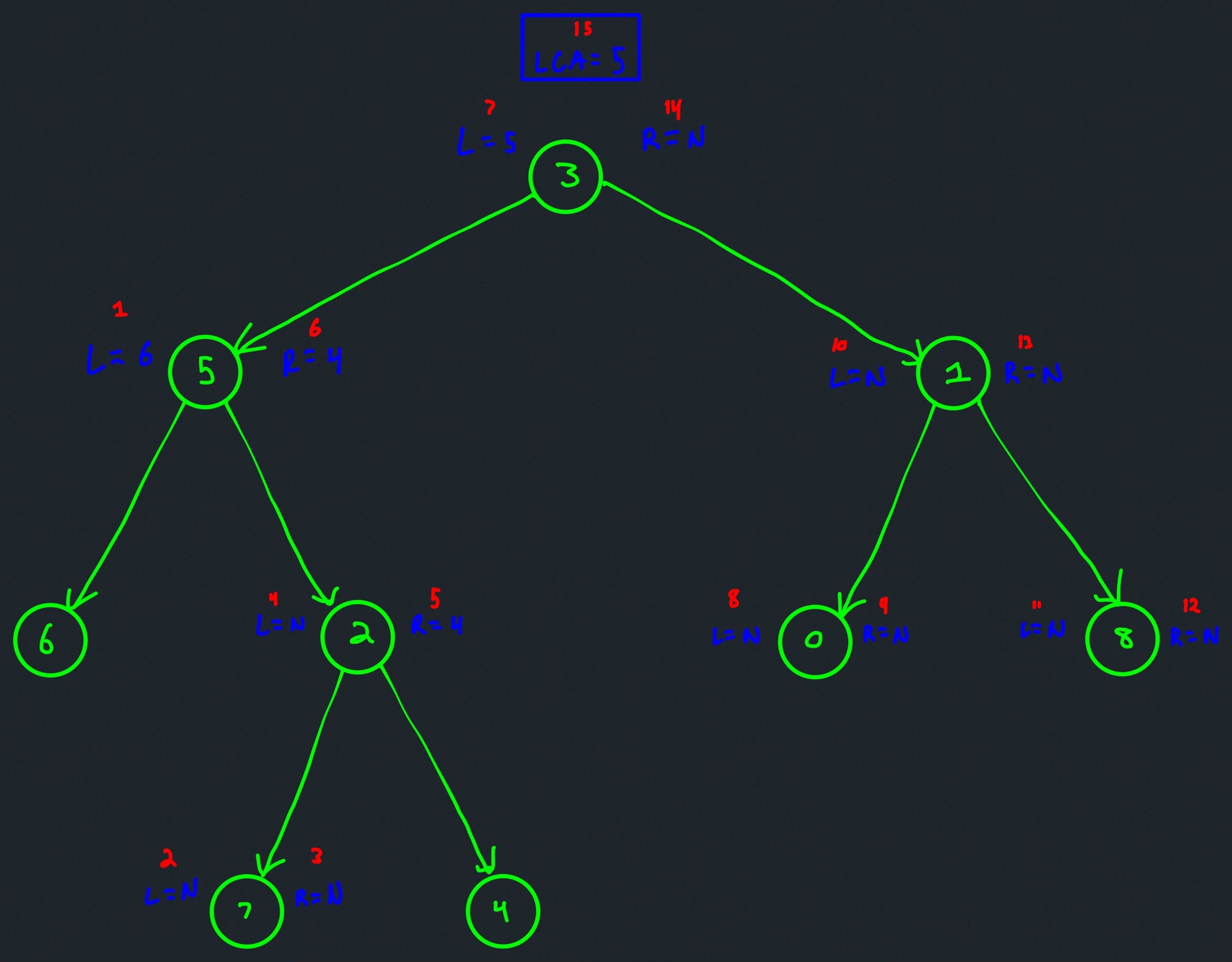
The image makes it clear how we do not continue processing a branch once a target node is found along that branch. Unfortunately, there's a clear inefficiency highlighted in the process pictured above — we still process the overall root's entire right subtree even though it's clearly not possible for the LCA to exist within it since both target nodes have already been found. Fixing this inefficiency would require a good bit more effort, but is worth considering at some point. The main goal of the picture is to illustrate how searches are executed and terminated and how values found are propagated back up the tree.
LC 111. Minimum Depth of Binary Tree (✓) ★★
Given a binary tree, find its minimum depth.
The minimum depth is the number of nodes along the shortest path from the root node down to the nearest leaf node.
Note: A leaf is a node with no children.
class Solution:
def minDepth(self, root: Optional[TreeNode]) -> int:
if not root:
return 0
if not root.left:
return 1 + self.minDepth(root.right)
elif not root.right:
return 1 + self.minDepth(root.left)
return 1 + min(self.minDepth(root.left), self.minDepth(root.right))
The inductive approach for this problem is not the easiest to come up with at first. The idea is that if the current node is missing its left child, then we should explore the right branch. If the current node is missing its right child, then we should explore the left branch. If neither child nodes are missing, then we should explore both branches. Whatever the case, the branch(es) we go down should have 1 added to it to account for the current node's depth.
The "traverse and accumulate" approach is easier to come up with but a bit of a cheat:
class Solution:
def minDepth(self, root: Optional[TreeNode]) -> int:
min_leaf_depth = float('inf')
def visit(node, curr_depth):
if not node and curr_depth > min_leaf_depth:
return
curr_depth += 1
nonlocal min_leaf_depth
if not node.left and not node.right:
min_leaf_depth = min(min_leaf_depth, curr_depth)
visit(node.left, curr_depth)
visit(node.right, curr_depth)
visit(root, 0)
return min_leaf_depth
LC 1026. Maximum Difference Between Node and Ancestor (✓)
Given the root of a binary tree, find the maximum value V for which there exist different nodes A and B where V = |A.val - B.val| and A is an ancestor of B.
A node A is an ancestor of B if either: any child of A is equal to B, or any child of A is an ancestor of B.
class Solution:
def maxAncestorDiff(self, root: Optional[TreeNode]) -> int:
def visit(node, max_path_val, min_path_val, max_diff_so_far):
if not node:
return max_path_val - min_path_val
max_path_val = max(max_path_val, node.val)
min_path_val = min(min_path_val, node.val)
left = visit(node.left, max_path_val, min_path_val, max_diff_so_far)
right = visit(node.right, max_path_val, min_path_val, max_diff_so_far)
return max(left, right)
return visit(root, float('-inf'), float('inf'), float('-inf'))
We're guaranteed at least two nodes which means we don't have to worry about edge cases as much. Our goal is basically to keep track of each path's maximum value as well as its minimum value because the maximum difference will be obtained by subtracting the minimum node value from the maximum node value.
LC 938. Range Sum of BST (✓)
Given the root node of a binary search tree, return the sum of values of all nodes with a value in the range [low, high].
class Solution:
def rangeSumBST(self, root: Optional[TreeNode], low: int, high: int) -> int:
if not root:
return 0
ans = 0
if low <= root.val <= high:
ans += root.val
if root.val > low:
ans += self.rangeSumBST(root.left, low, high)
if root.val < high:
ans += self.rangeSumBST(root.right, low, high)
return ans
We add the current node's value to the final answer in the pre-order stage of the traversal if the value falls in the [low, high] interval. How should we strategically visit the other subtrees though? We should make use of the fact that the tree is a BST. If the current node's value is less than low, then looking at the left subtree would be pointless because all of its values are less than the current node (because the tree is a BST); similarly, if the current node's value is greater than high, then looking at the right subtree would be pointless becall all of its values are greater than the current node (because the tree is a BST).
Great, so we know what not to do, but what should we do? If the current value is greater than low, then smaller values than the current value might be able to contribute to the range sum as well; hence, we should explore the left subtree. Similarly, if the current value is less than high, then larger values than the current value might be able to contribute to the range sum as well; hence, we should explore the right subtree. This lets us take advantage of the BST properties of the tree while efficiently performing a DFS traversal.
The solution above works in terms of how the answer is accumulate because we're only ever adding non-zero values if the value is in the range [low, high] or 0 otherwise. Thus, the final answer returned will be the desired range sum.
LC 101. Symmetric Tree (✓) ★★
Given a binary tree, check whether it is a mirror of itself (ie, symmetric around its center).
For example, this binary tree [1,2,2,3,4,4,3] is symmetric:
1
/ \
2 2
/ \ / \
3 4 4 3
But the following [1,2,2,null,3,null,3] is not:
1
/ \
2 2
\ \
3 3
class Solution:
def isSymmetric(self, root: Optional[TreeNode]) -> bool:
def dfs(node1, node2):
if not node1 and not node2:
return True
if not node1 or not node2 or node1.val != node2.val:
return False
return dfs(node1.left, node2.right) and dfs(node1.right, node2.left)
return dfs(root, root)
The solution above is not the easiest to come up with at first. In many ways, this problem resembles LC 100. Same Tree. Compare the solutions:
class Solution:
def isSameTree(self, p: Optional[TreeNode], q: Optional[TreeNode]) -> bool:
if not p and not q:
return True
if not p or not q or p.val != q.val:
return False
left = self.isSameTree(p.left, q.left)
right = self.isSameTree(p.right, q.right)
return left and right
The idea is that our DFS needs to be acting on the same node each time in two different ways — the left subtree of a node needs to mirror that same node's right subtree. This becomes possible when we allow our DFS function to receive two nodes as parameters.
The more intuitive, albeit slightly messier, approach is a modified BFS:
class Solution:
def isSymmetric(self, root: Optional[TreeNode]) -> bool:
def test_level(level_nodes):
l = 0
r = len(level_nodes) - 1
while l < r:
left = level_nodes[l]
right = level_nodes[r]
l += 1
r -= 1
if not left and not right:
continue
if (left and not right) or (right and not left) or left.val != right.val:
return False
return True
queue = deque([root])
while queue:
if not test_level(queue):
return False
num_nodes_this_level = len(queue)
for _ in range(num_nodes_this_level):
node = queue.popleft()
if node:
queue.append(node.left)
queue.append(node.right)
return True
The idea here is that we always push a node's children to the queue. We do this even if one of the children does not exist to ensure positions are maintained. Mirrored nodes to be equidistant from each other. Note that the lines
num_nodes_this_level = len(queue)
for _ in range(num_nodes_this_level):
are critical in the function above to ensure the test_level function is run only when an entire level has been enqueued.
LC 1325. Delete Leaves With a Given Value (✓) ★★
Given a binary tree root and an integer target, delete all the leaf nodes with value target.
Note that once you delete a leaf node with value target, if it's parent node becomes a leaf node and has the value target, it should also be deleted (you need to continue doing that until you can't).
class Solution:
def removeLeafNodes(self, root: Optional[TreeNode], target: int) -> Optional[TreeNode]:
if not root:
return None
root.left = self.removeLeafNodes(root.left, target)
root.right = self.removeLeafNodes(root.right, target)
if not root.left and not root.right and root.val == target:
return None
return root
This is a tough one at first, but we can use the DFS to reconstruct the tree, one node at a time, where leaf nodes are removed in the post-order stage of the traversal.
LC 235. Lowest Common Ancestor of a Binary Search Tree (✓) ★
Given a binary search tree (BST), find the lowest common ancestor (LCA) of two given nodes in the BST.
According to the definition of LCA on Wikipedia: "The lowest common ancestor is defined between two nodes p and q as the lowest node in T that has both p and q as descendants (where we allow a node to be a descendant of itself)."
class Solution:
def lowestCommonAncestor(self, root: 'TreeNode', p: 'TreeNode', q: 'TreeNode') -> 'TreeNode':
parent_val = root.val
p_val = p.val
q_val = q.val
# both p and q are greater than parent (LCA must be in right subtree of parent)
if p_val > parent_val and q_val > parent_val:
return self.lowestCommonAncestor(root.right, p, q)
# both p and q are less than parent (LCA must be in left subtree of parent)
elif p_val < parent_val and q_val < parent_val:
return self.lowestCommonAncestor(root.left, p, q)
# the current root must be the LCA because it is the split point
else:
return root
If we're familiar with the Lowest Common Ancestor problem, then it may seem like the tree being a BST will complicate things. But, in fact, the tree being a BST drastically simplifies the solution, as can be seen above. The following solution is the solution to the standard problem where the tree is not guaranteed to be a BST:
class Solution:
def lowestCommonAncestor(self, root: 'TreeNode', p: 'TreeNode', q: 'TreeNode') -> 'TreeNode':
if not root:
return None
if root == p or root == q:
return root
left = self.lowestCommonAncestor(root.left, p, q)
right = self.lowestCommonAncestor(root.right, p, q)
if left and right:
return root
return left if left else right
And with comments:
class Solution:
def lowestCommonAncestor(self, root: 'TreeNode', p: 'TreeNode', q: 'TreeNode') -> 'TreeNode':
# non-existent node cannot be LCA
if not root:
return None
# current node is p or q -- return it because it could be the LCA (pre-order at this point)
# stop searching further down this branch because the LCA cannot be deeper
# any lower node along this branch would not be an ancestor to both p and q
if root == p or root == q:
return root
left = self.lowestCommonAncestor(root.left, p, q)
right = self.lowestCommonAncestor(root.right, p, q)
# all child nodes of current node have been visited (post-order at this point)
# left/right will only hold non-null values if p or q (or both) were encountered
# (as children of the current node)
# if left AND right are non-null, then LCA must be current node
# (it serves as the connector between the two subtrees containing p and q)
if left and right:
return root
# both target nodes were not found in the current node's subtrees
# either one target was found (return that node) or no target was found
# (arbitrarily return right which will equal None)
return left if left else right
LC 450. Delete Node in a BST (✓) ★★★★
Given a root node reference of a BST and a key, delete the node with the given key in the BST. Return the root node reference (possibly updated) of the BST.
Basically, the deletion can be divided into two stages:
- Search for a node to remove.
- If the node is found, delete the node.
Follow up: Can you solve it with time complexity O(height of tree)?
class Solution:
# One step right and then always left
def successor(self, root: TreeNode) -> int:
root = root.right
while root.left:
root = root.left
return root.val
# One step left and then always right
def predecessor(self, root: TreeNode) -> int:
root = root.left
while root.right:
root = root.right
return root.val
def deleteNode(self, root: TreeNode, key: int) -> TreeNode:
if not root:
return None
# delete from the right subtree
if key > root.val:
root.right = self.deleteNode(root.right, key)
# delete from the left subtree
elif key < root.val:
root.left = self.deleteNode(root.left, key)
# delete the current node
else:
# the node is a leaf
if not (root.left or root.right):
root = None
# The node is not a leaf and has a right child
elif root.right:
root.val = self.successor(root)
root.right = self.deleteNode(root.right, root.val)
# the node is not a leaf, has no right child, and has a left child
else:
root.val = self.predecessor(root)
root.left = self.deleteNode(root.left, root.val)
return root
The solution above is straight from LeetCode's solution editorial. It is posted as a reminder to come back to it at another date, mostly due to the following comment:
The solution seems to clone the value at successor or predecessor instead of actually moving either of them up the tree at all. An interviewer can reasonably argue that this is not actually deleting a node because the node remains in the tree with an updated value from either predecessor or successor.
That is, the provided solution does not actually delete the node but simply overwrites values of other nodes to fulfill the BST property. One user refers people on to Java code from Sedgewick's famed algorithms text.
This would be a good problem to come back to.
Traverse-and-accumulate (visit nodes and accumulate information in nonlocal variables)
Remarks
Core idea: Visit all the nodes with a traversal and accumulate the wanted information in a nonlocal variable.
If we need to accumulate some global information about the entire tree, then we can use the this template to facilitate that process. This template is like doing a for loop through all the nodes, which is often very convenient. It would be great to be able to simply do
initialize some data
for node in tree:
do_something(node)
The traverse-and-accumulate template is basically a way to achieve this. It doesn't look like a for loop, because it uses recursion, but it can be used like a for loop. Furthermore, we can essentially do a for loop through the nodes in different orders depending on the traversal.
The parameter of the recursive function in the induction template is called root. This makes sense because
each node, when visited, is treated as the root of its own subtree. However, when using the
traverse-and-accumulate template, the parameter is called node instead of root. This is
because we think of it as just a for loop through the nodes, and we wouldn't do for root in tree: ....
The induction and traverse-and-accumulate templates can be mixed together with pre/in/postorder traversals on occasion, depending on the problem (such as LC 543. Diameter of Binary Tree).
Note (traversal ordering): The traverse-and-accumulate template, as presented below, uses a pre-order traversal since the updating of res (i.e., the processing of node by the visit function) occurs before processing the left or right subtrees with visit(node.left) and visit(node.right), respectively. We can modify the order of the traversal based on when/where we update res.
Note (traversal function name): Below, we use the function name visit to indicate how each node will be visited, starting from the root. A DFS traversal is implied, meaning we are going to use a pre-order, post-order, or in-order traversal of the tree to obtain our desired result. The contents of visit will make clear which traversal is being used. While visit is the function name used below, it's somewhat common for people to use dfs, process, or some other function name instead.
def solution(root):
res = ... # initial value
def visit(node):
if not node:
return
nonlocal res
res = ... # update res here
visit(node.left)
visit(node.right)
visit(root)
return res
Examples
Maximum difference between two nodes in a binary tree (not on LeetCode)
def max_diff(root):
if not root:
return 0
min_val = float('inf')
max_val = float('-inf')
def visit(node):
if not node:
return
nonlocal min_val, max_val
min_val = min(min_val, node.val)
max_val = max(max_val, node.val)
visit(node.left)
visit(node.right)
visit(root)
return max_val - min_val
The largest difference between nodes could be between nodes deeper down in the left and right subtrees of the tree's overall root; that is, we cannot effectively determine the answer for the whole tree from the answers for the subtrees. The induction template is thus not applicable. We can traverse and accumulate the overall maximum and minimum node values in non-local variables min_val and max_val. We report the answer after a full traversal by returning the difference between these values.
Longest unival vertical path (not on LeetCode)
def longest_vertical_path(root):
longest_path = 0
def visit(node, curr_path_val, curr_path_length):
if not node:
return
nonlocal longest_path
if node.val == curr_path_val:
curr_path_length += 1
longest_path = max(longest_path, curr_path_length)
else:
curr_path_length = 0
visit(node.left, node.val, curr_path_length)
visit(node.right, node.val, curr_path_length)
visit(root, root.val, 0)
return longest_path
The idea is to keep track of the longest univalue vertical path found so far by storing it in a nonlocal variable, longest_path. To calculate the longest vertical path for any given node, we pass that node's value down the tree as well as the current path length where that is the only value encountered thus far.
Find mode of a binary tree (not on LeetCode)
def tree_mode(root):
freqs = defaultdict(int)
max_freq = 0
mode = -1
def visit(node):
if not node:
return
nonlocal mode, max_freq
freqs[node.val] += 1
curr_freq = freqs[node.val]
max_freq = max(max_freq, curr_freq)
if curr_freq == max_freq:
mode = node.val
visit(root)
return mode
Since it's possible the mode may be a value that appears once or more in both subtrees, the induction template is not enough here. The approach above makes use of a hash map as a frequency lookup to progressively determine what the mode will be. It's also possible to determine the mode by passing information down the tree (although this approach is arguably less clear than the approach above):
def tree_mode(root):
freqs = defaultdict(int)
def visit(node, mode_so_far):
if not node:
return
freqs[node.val] += 1
mode_so_far = max(freqs[mode_so_far], freqs[node.val])
visit(node.left, mode_so_far)
visit(node.right, mode_so_far)
return mode_so_far
return visit(root, root.val)
LC 94. Binary Tree Inorder Traversal
Given the root of a binary tree, return the inorder traversal of its nodes' values.
class Solution:
def inorderTraversal(self, root: Optional[TreeNode]) -> List[int]:
node_vals = []
def visit(node):
if not node:
return
visit(node.left)
node_vals.append(node.val)
visit(node.right)
visit(root)
return node_vals
LC 144. Binary Tree Preorder Traversal
Given the root of a binary tree, return the preorder traversal of its nodes' values.
class Solution:
def preorderTraversal(self, root: Optional[TreeNode]) -> List[int]:
node_vals = []
def visit(node):
if not node:
return
node_vals.append(node.val)
visit(node.left)
visit(node.right)
visit(root)
return node_vals
LC 145. Binary Tree Postorder Traversal
Given the root of a binary tree, return the postorder traversal of its nodes' values.
class Solution:
def postorderTraversal(self, root: Optional[TreeNode]) -> List[int]:
node_vals = []
def visit(node):
if not node:
return
visit(node.left)
visit(node.right)
node_vals.append(node.val)
visit(root)
return node_vals
LC 98. Validate Binary Search Tree★
Given the root of a binary tree, determine if it is a valid binary search tree (BST).
A valid BST is defined as follows:
- The left subtree of a node contains only nodes with keys less than the node's key.
- The right subtree of a node contains only nodes with keys greater than the node's key.
- Both the left and right subtrees must also be binary search trees.
class Solution:
def isValidBST(self, root: Optional[TreeNode]) -> bool:
is_bst = True
prev = float('-inf')
def visit(node):
nonlocal is_bst, prev
if not node or not is_bst:
return
visit(node.left)
if prev >= node.val:
is_bst = False
prev = node.val
visit(node.right)
visit(root)
return is_bst
The solution above is slick in terms of how it uses prev to bypass adding a bunch of space overhead to the solution. It's sort of "linked list-ish" in nature in terms of how the prev "pointer" is being used and updated. A more obvious solution that results in adding a bunch of space is as follows (this just assembles the array of node values and we check to see if it is sorted or not — both solutions are for time and space, but the solution above is more elegant):
class Solution:
def isValidBST(self, root: Optional[TreeNode]) -> bool:
node_vals = []
def visit(node):
if not node:
return
visit(node.left)
node_vals.append(node.val)
visit(node.right)
visit(root)
for i in range(1, len(node_vals)):
if node_vals[i - 1] >= node_vals[i]:
return False
return True
LC 530. Minimum Absolute Difference in BST
Given a binary search tree with non-negative values, find the minimum absolute difference between values of any two nodes.
class Solution:
def getMinimumDifference(self, root: Optional[TreeNode]) -> int:
min_diff = float('inf')
prev = float('-inf')
def visit(node):
if not node:
return
visit(node.left)
nonlocal min_diff, prev
min_diff = min(min_diff, node.val - prev)
prev = node.val
visit(node.right)
return node.val
visit(root)
return min_diff
The key realization here is that an in-order traversal gives us the node values in sorted ascending order. Hence, we can make use of a prev variable to store the value of previous nodes and we compare adjacent nodes as we go, keeping track of the minimum difference encountered, min_diff, along the way. In the code above, note that min_diff and prev are initialized in ways that ensure calculations are meaningful for two or more nodes, which we're guaranteed to have in this problem.
LC 1038. Binary Search Tree to Greater Sum Tree
Given the root of a Binary Search Tree (BST), convert it to a Greater Tree such that every key of the original BST is changed to the original key plus sum of all keys greater than the original key in BST.
As a reminder, a binary search tree is a tree that satisfies these constraints:
- The left subtree of a node contains only nodes with keys less than the node's key.
- The right subtree of a node contains only nodes with keys greater than the node's key.
- Both the left and right subtrees must also be binary search trees.
Note: This question is the same as 538: https://leetcode.com/problems/convert-bst-to-greater-tree/
class Solution:
def bstToGst(self, root: TreeNode) -> TreeNode:
sum_so_far = 0
def visit(node):
if not node:
return
visit(node.right)
nonlocal sum_so_far
sum_so_far += node.val
node.val = sum_so_far
visit(node.left)
visit(root)
return root
First recall that a conventional (i.e., left to right) in-order traversal of a BST results in traversing the nodes in sorted ascending order. Sometimes, like in this problem, it helps to execute an in-order traversal from right to left, which will yield values in sorted descending order. This realization makes this problem much easier to approach. Execute a right to left in-order traversal and update each node's value to sum_so_far, an accumulated sum of all node values reached thus far.
LC 700. Search in a Binary Search Tree
You are given the root of a binary search tree (BST) and an integer val.
Find the node in the BST that the node's value equals val and return the subtree rooted with that node. If such a node does not exist, return null.
class Solution:
def searchBST(self, root: Optional[TreeNode], val: int) -> Optional[TreeNode]:
target_node = None
def visit(node):
nonlocal target_node
if not node or target_node:
return
if node.val > val:
visit(node.left)
elif node.val < val:
visit(node.right)
else:
target_node = node
visit(root)
return target_node
This problem has an easy solution if you don't take advantage of the fact that the tree is a BST:
class Solution:
def searchBST(self, root: Optional[TreeNode], val: int) -> Optional[TreeNode]:
target_node = None
def visit(node):
nonlocal target_node
if not node or target_node:
return
if node.val == val:
target_node = node
visit(node.left)
visit(node.right)
visit(root)
return target_node
But that's not the point of the problem. Only a small adjustment needs to be made in order to really take advantage of the fact that the tree is a BST. Only visit a node in a subsequent subtree if it's possible for that subtree to have the node.
LC 701. Insert into a Binary Search Tree
You are given the root node of a binary search tree (BST) and a value to insert into the tree. Return the root node of the BST after the insertion. It is guaranteed that the new value does not exist in the original BST.
Notice that there may exist multiple valid ways for the insertion, as long as the tree remains a BST after insertion. You can return any of them.
class Solution:
def insertIntoBST(self, root: Optional[TreeNode], val: int) -> Optional[TreeNode]:
if not root:
return TreeNode(val)
ref_node_found = False
def visit(node):
nonlocal ref_node_found
if not node or ref_node_found:
return
if not node.left and val < node.val:
node.left = TreeNode(val)
ref_node_found = True
if not node.right and val > node.val:
node.right = TreeNode(val)
ref_node_found = True
if node.val < val:
visit(node.right)
else:
visit(node.left)
visit(root)
return root
The idea in the solution above is to traverse the BST by taking advantage of its BST nature — we only consider inserting the node when there's a natural opportunity to do so (i.e., when the current node is missing its left or right child). We use ref_node_found to optimize for an early return.
The inductive alternative for solving this problem is more arguably more elegant but harder to envision at first:
class Solution:
def insertIntoBST(self, root: Optional[TreeNode], val: int) -> Optional[TreeNode]:
if not root:
return TreeNode(val)
if val > root.val:
root.right = self.insertIntoBST(root.right, val)
if val < root.val:
root.left = self.insertIntoBST(root.left, val)
return root
LC 270. Closest Binary Search Tree Value★
Given the root of a binary search tree and a target value, return the value in the BST that is closest to the target.
class Solution:
def closestValue(self, root: Optional[TreeNode], target: float) -> int:
closest = root.val
curr_diff = abs(closest - target)
def visit(node):
nonlocal closest, curr_diff
if not node:
return
diff = abs(node.val - target)
if diff <= curr_diff:
if diff != curr_diff:
curr_diff = diff
closest = node.val
else:
closest = min(closest, node.val)
if target > node.val:
visit(node.right)
elif target < node.val:
visit(node.left)
else:
closest = node.val
visit(root)
return closest
The solution above is, oddly enough, probably the easiest of the approaches to come up with where we're both taking advantage of the BST tree structure as well as not allocating additional space beyond the call stack for the recursion.
If, however, we allow ourselves the freedom to perform an in-order traversal where we just assemble a sorted array ( additional space to store all the node values), then we can easily iterate through the sorted array to find the closest value:
class Solution:
def closestValue(self, root: TreeNode, target: float) -> int:
def inorder(node):
return inorder(node.left) + [node.val] + inorder(node.right) if node else []
return min(inorder(root), key = lambda x: abs(target - x))
This is cute and short but not particularly clever since we create an array the full size of the tree just to store the node values when that's really unnecessary.
LC 1448. Count Good Nodes in Binary Tree (✓)
Given a binary tree root, a node X in the tree is named good if in the path from root to X there are no nodes with a value greater than X.
Return the number of good nodes in the binary tree.
class Solution:
def goodNodes(self, root: TreeNode) -> int:
good_nodes = 0
def visit(node, max_so_far):
nonlocal good_nodes
if not node:
return
max_so_far = max(max_so_far, node.val)
if node.val >= max_so_far:
good_nodes += 1
visit(node.left, max_so_far)
visit(node.right, max_so_far)
visit(root, root.val)
return good_nodes
We traverse the tree and accumulate the number of good nodes in the nonlocal good_nodes variable — keeping track of the max_so_far for the maximum node value in a path is how we determine for each node we encounter whether or not that node should be considered good. We use a pre-order traversal to accomplish this.
The induction alternative is also quite possible but arguably more difficult to come up with at first (it uses a post-order traversal and starts adding values to the total number of good nodes once we hit a leaf and then adds values as we backtrack back up the path):
class Solution:
def goodNodes(self, root: TreeNode) -> int:
def visit(node, max_so_far):
if not node:
return 0
left = visit(node.left, max(max_so_far, node.val))
right = visit(node.right, max(max_so_far, node.val))
ans = left + right
if node.val >= max_so_far:
ans += 1
return ans
return visit(root, float("-inf"))
LC 111. Minimum Depth of Binary Tree (✓)
Given a binary tree, find its minimum depth.
The minimum depth is the number of nodes along the shortest path from the root node down to the nearest leaf node.
Note: A leaf is a node with no children.
class Solution:
def minDepth(self, root: Optional[TreeNode]) -> int:
min_leaf_depth = float('inf')
def visit(node, curr_depth):
if not node and curr_depth > min_leaf_depth:
return
curr_depth += 1
nonlocal min_leaf_depth
if not node.left and not node.right:
min_leaf_depth = min(min_leaf_depth, curr_depth)
visit(node.left, curr_depth)
visit(node.right, curr_depth)
visit(root, 0)
return min_leaf_depth
The approach above is really quite simple. The pure inductive approach is a bit harder to come up with but rather elegant:
class Solution:
def minDepth(self, root: Optional[TreeNode]) -> int:
if not root:
return 0
if not root.left:
return 1 + self.minDepth(root.right)
elif not root.right:
return 1 + self.minDepth(root.left)
return 1 + min(self.minDepth(root.left), self.minDepth(root.right))
LC 199. Binary Tree Right Side View (✓)
Given the root of a binary tree, imagine yourself standing on the right side of it, return the values of the nodes you can see ordered from top to bottom.
class Solution:
def rightSideView(self, root: Optional[TreeNode]) -> List[int]:
if not root:
return root
level_node_vals_rightmost = []
def visit(node, level):
if not node:
return
if level == len(level_node_vals_rightmost):
level_node_vals_rightmost.append(node.val)
visit(node.right, level + 1)
visit(node.left, level + 1)
visit(root, 0)
return level_node_vals_rightmost
The BFS approach to this problem is a bit clearer to envision, but a clever DFS solution is also quite possible, as evidenced above. Specifically, this problem is an excellent illustration of where logic in the pre-order stage of a traversal can be very helpful. The right side view dictates that we always report the value of the rightmost node for each level of the tree. We're not guaranteed that each node will have a right child. For some levels, a node's left child may actually be the level's rightmost node whose value we need to report. The key insight is to use a right-to-left traversal where in the pre-order stage we determine whether or not the current node's value should be added to the list we're ultimately trying to return — we cleverly use the length of the list to determine whether or not a node's value should be added.
LC 872. Leaf-Similar Trees (✓)
Consider all the leaves of a binary tree, from left to right order, the values of those leaves form a leaf value sequence.
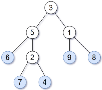
For example, in the given tree above, the leaf value sequence is (6, 7, 4, 9, 8).
Two binary trees are considered leaf-similar if their leaf value sequence is the same.
Return true if and only if the two given trees with head nodes root1 and root2 are leaf-similar.
class Solution:
def leafSimilar(self, root1: Optional[TreeNode], root2: Optional[TreeNode]) -> bool:
def dfs(node, leaf_vals):
if not node:
return
if not node.left and not node.right:
leaf_vals.append(node.val)
dfs(node.left, leaf_vals)
dfs(node.right, leaf_vals)
return leaf_vals
t1_leaf_vals = dfs(root1, [])
t2_leaf_vals = dfs(root2, [])
if len(t1_leaf_vals) != len(t2_leaf_vals):
return False
for i in range(len(t1_leaf_vals)):
if t1_leaf_vals[i] != t2_leaf_vals[i]:
return False
return True
The core idea above is to traverse each tree, accumulating the leaf values in each and then compare those values. Another more nifty and Pythonic approach is as follows:
class Solution:
def leafSimilar(self, root1, root2):
def dfs(node):
if node:
if not node.left and not node.right:
yield node.val
yield from dfs(node.left)
yield from dfs(node.right)
return list(dfs(root1)) == list(dfs(root2))
LC 113. Path Sum II (✓) ★
Given the root of a binary tree and an integer targetSum, return all root-to-leaf paths where each path's sum equals targetSum.
A leaf is a node with no children.
class Solution:
def pathSum(self, root: Optional[TreeNode], targetSum: int) -> List[List[int]]:
paths = []
def dfs(node, sum_so_far, path_vals):
if not node:
return
sum_so_far += node.val
path_vals.append(node.val)
if sum_so_far == targetSum and not node.left and not node.right:
paths.append(path_vals[:])
dfs(node.left, sum_so_far, path_vals)
dfs(node.right, sum_so_far, path_vals)
path_vals.pop()
dfs(root, 0, [])
return paths
This is a lovely problem, especially for the traverse-and-accumulate template. The main wrinkle is the need for the backtracking bit: path_vals.pop(). This line occurs after the subtree for a node has been processed and that node should be removed from consideration for a path. Another potential gotcha is the line once the target sum has been reached at a leaf node: paths.append(path_vals[:]). If, instead, we had paths.append(path_vals), then we'd encounter some errors because path_vals is a list which means it is mutable, but we do not want to mutate the list we end up pushing to paths; hence, we make a copy of path_vals when the target sum is reached and we push that copy to paths.
LC 437. Path Sum III (✓) ★★★
You are given a binary tree in which each node contains an integer value.
Find the number of paths that sum to a given value.
The path does not need to start or end at the root or a leaf, but it must go downwards (traveling only from parent nodes to child nodes).
The tree has no more than 1,000 nodes and the values are in the range -1,000,000 to 1,000,000.
class Solution:
def pathSum(self, root: Optional[TreeNode], targetSum: int) -> int:
def dfs(node, path_sum):
if not node:
return
nonlocal ans
path_sum += node.val
ans += counts[path_sum - targetSum]
counts[path_sum] += 1
dfs(node.left, path_sum)
dfs(node.right, path_sum)
counts[path_sum] -= 1
counts = defaultdict(int)
counts[0] = 1
ans = 0
dfs(root, 0)
return ans
The solution above cleverly exploits the idea of a sort of progressive prefix sum where the frequency of prefix sums encountered is tracked in the counts hash map. The backtracking part counts[path_sum] -= 1 is important for once the current node is no longer part of the path sum (i.e., the frequency for that path sum should then be decremented by 1).
LC 1305. All Elements in Two Binary Search Trees (✓)
Given two binary search trees root1 and root2.
Return a list containing all the integers from both trees sorted in ascending order.
class Solution:
def getAllElements(self, root1: TreeNode, root2: TreeNode) -> List[int]:
def merge_sorted_arrs(arr1, arr2):
merged = []
p1 = p2 = 0
while p1 < len(arr1) and p2 < len(arr2):
num1 = arr1[p1]
num2 = arr2[p2]
if num1 < num2:
merged.append(num1)
p1 += 1
elif num1 > num2:
merged.append(num2)
p2 += 1
else:
merged.append(num1)
merged.append(num2)
p1 += 1
p2 += 1
while p1 < len(arr1):
merged.append(arr1[p1])
p1 += 1
while p2 < len(arr2):
merged.append(arr2[p2])
p2 += 1
return merged
def dfs(node, sorted_vals):
if not node:
return []
dfs(node.left, sorted_vals)
sorted_vals.append(node.val)
dfs(node.right, sorted_vals)
return sorted_vals
t1_vals = dfs(root1, [])
t2_vals = dfs(root2, [])
return merge_sorted_arrs(t1_vals, t2_vals)
This is a pretty dumb problem. At first, it makes you think there might be some fancy trick for obtaining the sorted list. Nope. An in-order DFS needs to be executed on both trees to obtain each tree's values in sorted order, and then those sorted lists need to be merged in sorted order. Lame.
Combining templates: induction and traverse-and-accumulate
Remarks
TLDR (use template for reference): The points directly below are elaborated on more extensively under the dividing line. Use the provided template for explicit reference. The general concepts are remarked on first and then their applicability to the template specifically is addressed.
- Parent to child data flow: Use recursive call parameters to pass information down the tree from parent to child. This means defining the
visitfunction with more than just thenodeparameter (we're not usually allowed to alter thesolutionfunction signature). The information passed down can be data passed by value or by reference (if the latter, be cautious of when state mutations should not be shared across different branches of the tree). - Child to parent data flow: Use the induction template. This means whatever function is being called recursively must actually return a value. Usually this means finding solutions for the subtrees is enough to find the solution for the entire tree — we solve the problem at the subtrees recursively and then aggregate the results at the root. For a pure induction template answer, this means
solutionreturns a value which builds or aggregates solutions from the leaves to the root. If the template usage needs to be mixed, then defining a helper function,visit, and returning a value from that function will be necessary. - Global access (non-parent-child data flow): Sometimes it is not enough (or overly cumbersome) to strictly communicate between parent and child, and we need to break out of the normal traversal order. We effectively visit all the nodes with a traversal while accumulating the wanted information in a nonlocal variable. If all we need to do is accumulate data in nonlocal variables, then it is unnecessary to return anything from the
visitfunction (i.e., a pure usage of the traverse-and-accumulate template); however, if we also need to pass information back up the tree, then we will need to rely on the induction template as well.
Note how everything above is concerned with how node data can flow as opposed to the order in which node data is encountered. The order in which node data is encountered and processed is determined by the various DFS traversals: pre-order, in-order, and post-order. But, in general, the direction of information flow (e.g., downward from parent to child) and the order of node processing (e.g., post-order) are separate aspects to consider when coming up with a tree traversal strategy. These aspects should be combined as needed or appropriate.
In general, which (DFS) tree traversal template you use to solve a problem largely depends on how you need to manage the information or data flow between nodes. Specifically, information can flow in the following ways:
-
Parent to child (recursive call parameters): We use the parameters of the recursive call when we need to pass information down the tree. This means we can visit or process the current
node(i.e., the "parent") and pass along data we'd like to have access to (via recursive call parameters) when we process its children (i.e.,node.leftandnode.right).Template usage: This means defining the
visitfunction with more than just thenodeparameter. For example, a very rough start of an implementation might look as follows:def visit(node, data_received_from_parent):
# ...
# update/use data_received_from_parent
visit(node.left, data_from_curr_node_to_its_left_child_node)
visit(node.right, data_from_curr_node_to_its_right_child_node)
# ...The data passed from parent to child does not need to be restricted to a single parameter as in the simple illustration above. Multiple parameters could be used depending on the problem.
Examples of potentially meaningful parameters might include data passed by value like
sum_so_far,curr_path_length,path_str, etc. (i.e., data that is immutable and passed by value such as a string, integer, etc.), where we can freely update these values to pass along in subsequent recursive calls without worrying about mutations (i.e., the state of the variable wouldn't be shared across different branches of the tree).The data could also be passed from parent to child by reference such as a list, dictionary, etc.. In such cases, we need to be aware of and make a decision about how we want the state of the referenced data to be managed. By default, the referenced data will be mutated and its state shared across different branches of the tree. Such mutations and state sharing across branches is often undesirable; hence, we need to effectively undo the state changes/mutations after the recursive calls. This will ensure the state is not shared across different branches of the tree. For example, if the data being passed down by reference is a list, and we're appending to the list before the recursive calls, then we should pop from the list after the recursive calls to return the referenced data to its original state before the recursion.
-
Child to parent (induction): We use the induction template when we need to pass information up the tree. We can use the "pure induction template" (i.e., no changes needed) if it suffices to solve the problem at hand by simply solving the problem for the subtrees (i.e., essentially building up the solution from the leaves to the root):
def solution(root):
if not root:
return ...
res_left = solution(root.left)
res_right = solution(root.right)
# return a value computed via res_left, res_right, and root.val
return ...If, however, the problem involves also needing to accumulate information in a nonlocal variable(s), then we'll need to make a slight change to use the induction template properly, namely by creating a helper function,
visit, and then returning values from within that function:def solution(root):
# ... (accumulation variables)
def visit(node):
if not node:
return ...
# ... (accumulation happens here)
res_left = visit(node.left)
res_right = visit(node.right)
# return a value computed via res_left, res_right, and node.val
return ...
visit(root)
return resWhatever the case, as can be seen above, when passing information up the tree (i.e., when we use any form of the induction template), we need to be returning values from the function that is being called recursively.
-
Global access (traverse-and-accumulate): Sometimes it is not enough (or overly cumbersome) to strictly communicate between parent and child, and we need to break out of the normal traversal order. We effectively visit all the nodes with a traversal while accumulating the wanted information in a nonlocal variable(s). If all we need to do is accumulate data in nonlocal variables, then it is unnecessary to return anything from the
visitfunction (i.e., a pure usage of the traverse-and-accumulate template):def solution(root):
res = ... # initial value for accumulation
def visit(node):
if not node:
return # no value needs to be returned
nonlocal res
res = ... # update accumulated value here
visit(node.left)
visit(node.right)
# no return value from visit function
visit(root)
return res # return the accumulated valueIf, however, we also need to pass information back up the tree, then we will need to rely on the induction template as well (note how we now need to return values from within the
visitfunction):def solution(root):
res = ... # initial value for accumulation
def visit(node):
if not node:
return ...
nonlocal res
res = ... # update accumulated value here
res_left = visit(node.left)
res_right = visit(node.right)
# return a value computed via res_left, res_right, and node.val
return ...
visit(root)
return res # return accumulated value
All of the observations above lead us to the combined template provided below.
Short version of template
def solution(root):
res = ... # initial value
def visit(node):
if not node:
return ...
nonlocal res
res = ... # update res here
res_left = visit(node.left)
res_right = visit(node.right)
# return a value computed via res_left, res_right, and node.val
return ...
visit(root)
return res
""" Function signature (something we cannot alter but can mimic altering via the visit function) """
def solution(root):
""" Accumulated values (traverse-and-accumulate)"""
acc_1 = ... # accumulated value 1
acc_2 = ... # accumulated value 2
acc_3 = ... # accumulated value 3
""" Pass data down via recursive call params """
def visit(node, data_pass_down_by_val, data_pass_down_by_ref):
if not node:
return ... # return nothing for early termination (traverse-and-accumulate) OR
# return data for base case or return early for termination (induction)
nonlocal acc_1, acc_2, acc_3 # access nonlocal variables for accumulation
acc_x = ... # update accumulated values
# update/use data_pass_down_by_val
# update/use data_pass_down_by_ref
left_subtree = visit(node.left, data_pass_down_by_val, data_pass_down_by_ref)
right_subtree = visit(node.right, data_pass_down_by_val, data_pass_down_by_ref)
# undo mutation to data_pass_down_by_ref
# (assuming the state should not be shared across different branches of the tree)
""" Pass data up (induction) """
return ... # return a value computed via left_subtree, right_subtree, and node.val
""" Execute tree traversal """
# pass info down and up while accumulating (starting at root)
visit(root, init_data_val, init_data_ref)
# return something based on accumulated values or induction result
return acc_x
Examples
Find height of a tree node (not on LeetCode)
def node_height(root, target):
target_height = -1
def visit(node):
if not node:
return -1
left_height = visit(node.left)
right_height = visit(node.right)
height = 1 + max(left_height, right_height)
if node.val == target:
nonlocal target_height
target_height = height
return height
visit(root)
return target_height
This problem assumes our tree is comprised of nodes with unique values. It helps to do a post-order traversal here, where we build the height up from the leaf nodes, and we only update the nonlocal target_height once the target value has been encountered for the node whose height we're trying to find.
Remember that a node's height is the longest path from the node to a leaf whereas a node's depth is the length of the path from the root of the tree to that node:
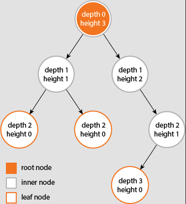
LC 543. Diameter of Binary Tree★★
Given the root of a binary tree, return the length of the diameter of the tree.
The diameter of a binary tree is the length of the longest path between any two nodes in a tree. This path may or may not pass through the root.
The length of a path between two nodes is represented by the number of edges between them.
class Solution:
def diameterOfBinaryTree(self, root: Optional[TreeNode]) -> int:
diameter = 0
def visit(node):
if not node:
return -1
left_height = visit(node.left)
right_height = visit(node.right)
nonlocal diameter
diameter = max(diameter, left_height + right_height + 2)
curr_height = 1 + max(left_height, right_height)
return curr_height
visit(root)
return diameter
This problem can be surprisingly difficult depending on how you look at it. Some contemplation results in thinking that the solution has to be related to finding the node whose combination of left and right subtree heights is maximal. Hence, much of the problem really boils down to being able to find the height of a subtree, where recall the height is the distance of the longest path from a node to a leaf. This is different than the depth, which always has the root as a reference point:
- depth of a node: number of edges from the root to that node
- height of a node: number of edges from that node to a leaf
- height of the tree: height of the root
It's informative to first figure out how to calculate the height of a node given that node's value and the root of the tree:
def node_height(root, target):
target_height = -1
def visit(node):
if not node:
return -1
left_height = visit(node.left)
right_height = visit(node.right)
height = 1 + max(left_height, right_height)
if node.val == target:
nonlocal target_height
target_height = height
return height
visit(root)
return target_height
The solution for the diameter problem is then strikingly similar, as the solution at the top shows. The problem description notes that the path determining the diameter may or may not pass through the root, where by root they're referring to the overall root of the tree. But of course the path determining the diameter must pass through some subtree's root. And that's the point. We want to find the combination of heights for left and right subtrees for any given node, add 2 to get the path length (we add 2 because the current node serves as the subtree's root, which is the connecting point for the left and right subtrees — we must add 2 to account for the edges that connect the left and right subtrees to their root, the current node), and we want to find the combination such that the overall length or edge count is maximal.
LC 563. Binary Tree Tilt★★
Given the root of a binary tree, return the sum of every tree node's tilt.
The tilt of a tree node is the absolute difference between the sum of all left subtree node values and all right subtree node values. If a node does not have a left child, then the sum of the left subtree node values is treated as 0. The rule is similar if there the node does not have a right child.
class Solution:
def findTilt(self, root: Optional[TreeNode]) -> int:
tilt = 0
def visit(node):
if not node:
return 0
left_sum = visit(node.left)
right_sum = visit(node.right)
nonlocal tilt
tilt += abs(left_sum - right_sum)
return left_sum + right_sum + node.val
visit(root)
return tilt
This can be a rather difficult problem at first given its unusual framing. Once it's clear what you're actually trying to accomplish, it becomes clear that a post-order traversal is really what's needed. We find the tilt from the leaves up, where each node serves as its own subtree's root.
The primary difficulty is arguably identifying what we need to pass back up the tree. Just passing node.val back up the tree will not let us accomplish the desired effect (we need a cumulative sum for each subtree as we move up from the leaves, not just individual node values). It's like we basically need to sum all nodes of a subtree and send that back up while we're going back up the tree.
The leaves can provide useful hints for these kinds of problems — if we're at a node that has two children which are both leaves, then how do we effectively capture both of these nodes' values to send back up the tree? We first need to find the tilt that the current node contributes to the overall tilt, and this is always done for the current node by subtracting its left subtree sum from its right subtree sum and adding the absolute difference to the overall tilt. Hence, we effectively need to keep track of all the left and right subtree sums and keep passing this information up the tree.
LC 110. Balanced Binary Tree★★
Given a binary tree, determine if it is height-balanced.
For this problem, a height-balanced binary tree is defined as:
a binary tree in which the left and right subtrees of every node differ in height by no more than 1.
class Solution:
def isBalanced(self, root: Optional[TreeNode]) -> bool:
if not root:
return True
max_height_diff = float('-inf')
def visit(node):
nonlocal max_height_diff
if not node or max_height_diff > 1:
return -1
left_height = visit(node.left)
right_height = visit(node.right)
max_height_diff = max(max_height_diff, abs(left_height - right_height))
height = 1 + max(left_height, right_height)
return height
visit(root)
return max_height_diff < 2
The idea is to use a post-order traversal where you start comparing left and right subtree heights from the bottom up. The nonlocal max_height_diff variable lets us keep track of the maximum difference in heights we've encountered from any given node. If max_height_diff ever exceeds 1, then we simply repurpose the base case of returning -1 as an early return (this is simply an optimization step — the solution works just fine if we remove or max_height_diff > 1 from the base case conditional).
LC 1372. Longest ZigZag Path in a Binary Tree (✓) ★★★
You are given the root of a binary tree.
A ZigZag path for a binary tree is defined as follow:
- Choose any node in the binary tree and a direction (right or left).
- If the current direction is right, move to the right child of the current node; otherwise, move to the left child.
- Change the direction from right to left or from left to right.
- Repeat the second and third steps until you can't move in the tree.
Zigzag length is defined as the number of nodes visited - 1. (A single node has a length of 0).
Return the longest ZigZag path contained in that tree.
class Solution:
def longestZigZag(self, root: Optional[TreeNode]) -> int:
path_length = 0
def dfs(node):
if not node:
return (0,0)
left = dfs(node.left)[0]
right = dfs(node.right)[1]
nonlocal path_length
path_length = max(path_length, left, right)
return (right + 1, left + 1)
dfs(root)
return path_length
This problem is a real doozy at first. The solution above is based on this excellent solution. The idea is to return values in a tuple in such a way that the path length keeps increasing by 1 (from the bottom due to the post-order traversal) so long as the zigzag pattern is maintained (the zigzag pattern is maintained by swapping the order of the returned values for each DFS call) or a value of 0 is returned, in which case the path length for that zigzag is effectively reset.
An illustrative example can help a great deal. Consider the following tree:
__2
/ \
3 12______
\ \
1 ____7_____
/ \
8__ ___5
\ / \
9 4 11
/ \
6 10
The tree above can be used as a test case on LeetCode by defining the tree as follows:
[2,3,12,null,1,null,7,null,null,8,5,null,9,4,11,6,null,null,10]
The longest zigzag path is 12 -> 7 -> 8 -> 9 -> 6 (right, left, right, left for a path length of 4). How is this path length actually calculated with the solution above though? Drawing a picture always helps:
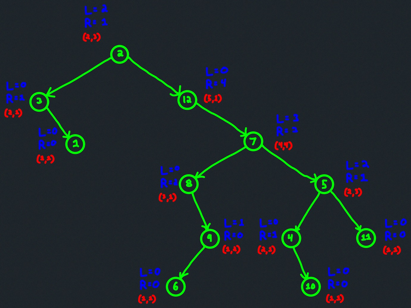
One thing to note about the image: the L and R value for each node is obtained by the tuple value returned by the left child at index 0 and the tuple value returned by the right child at index 1, respectively. For example, the node with value 5 has a left child that returns (2,1) and a right child that returns (1,1); hence, L and R for the node with value 5 is 2 from (2,1) and 1 from (1,1):
(2,1) (1,1)
L R
Adding a print statement right before the return within the dfs function can help clarify and confirm the process illustrated above:
print(f'Node: {node.val}; L = {left}; R = {right}; Return: ({right + 1},{left + 1})')
The following is printed to the console:
Node: 1; L = 0; R = 0; Return: (1,1)
Node: 3; L = 0; R = 1; Return: (2,1)
Node: 6; L = 0; R = 0; Return: (1,1)
Node: 9; L = 1; R = 0; Return: (1,2)
Node: 8; L = 0; R = 2; Return: (3,1)
Node: 10; L = 0; R = 0; Return: (1,1)
Node: 4; L = 0; R = 1; Return: (2,1)
Node: 11; L = 0; R = 0; Return: (1,1)
Node: 5; L = 2; R = 1; Return: (2,3)
Node: 7; L = 3; R = 3; Return: (4,4)
Node: 12; L = 0; R = 4; Return: (5,1)
Node: 2; L = 2; R = 1; Return: (2,3)
This confirms everything illustrated in the image. Note that since path_length is calculated as path_length = max(path_length, left, right) before the tuple return (right + 1, left + 1), we can see from the above that our final maximum path_length value is 4 (one unit less than 5).
Two pointers
Opposite ends
Remarks
The idea behind the "opposite ends" two pointer template is to move from the extremes (i.e., beginning and end) toward each other. Binary search is a class example of this template in action.
The template guarantees an run time because only iterations of the while loop may occur — the left and right pointers begin units away from each other and move at least one step closer to each other on every iteration. If the work inside each iteration is kept to , then the result will be an run time.
def fn(arr):
left = 0
right = len(arr) - 1
while left < right:
# choose one of the following depending on the problem:
# left += 1
# right -= 1
# increment left AND decrement right: left += 1 AND right -= 1
Examples
Determine if a string is a palindrome (✓)
def check_if_palindrome(s):
left = 0
right = len(s) - 1
while left < right:
if s[left] != s[right]:
return False
left += 1
right -= 1
return True
Note that for odd-length s the middle character is not actually processed and that's okay.
Time: . This algorithm is where is the length of the string s. We cannot make more iterations than the length of s since we either return false or increment and decrement at the same time. In actuality, the time is closer to .
Space: . A constant amount of memory is allocated.
Determine if a pair of integers sums to a target in a sorted array of unique integers (✓)
def check_for_target(nums, target):
left = 0
right = len(nums) - 1
while left < right:
pair_sum = nums[left] + nums[right]
if pair_sum > target: # pair_sum is too large (decrease by decrementing right pointer)
right -= 1
elif pair_sum < target: # pair_sum is too small (increase by incremeneting left pointer)
left += 1
else:
return True # pair_sum equals target (return True)
return False
The important observation here is that the pair sum can only increase by incrementing the left pointer while it can only decrease by decrementing the right pointer (due to the sorted nature of the input array, nums). Additionally worth noting is the need for the strict inequality left < right; if the inequality were not strict, then we could consider the same unique element twice (i.e., when left == right), which is not desired.
Time: . The left and right pointers start a distance from each other, where is the length of nums, and these pointers work their way towards each other for the duration of the while loop. We cannot have more than iterations.
Space: . Only a constant amount of memory allocation is used.
LC 344. Reverse String (✓, ✠)
Write a function that reverses a string. The input string is given as an array of characters s.
class Solution:
def reverseString(self, s: List[str]) -> None:
"""
Do not return anything, modify s in-place instead.
"""
left = 0
right = len(s) - 1
while left < right:
s[left], s[right] = s[right], s[left]
left += 1
right -= 1
Keep swapping characters until left is equal to or greater than right. Note that for odd-length s the middle character is not actually processed and that's okay since all other characters have been swapped.
The solution above takes advantage of Python's tuple unpacking/simultaneous assignment, but a more conventional approach where we rely on a temp variable would be as follows:
class Solution:
def reverseString(self, s: List[str]) -> None:
"""
Do not return anything, modify s in-place instead.
"""
left = 0
right = len(s) - 1
while left < right:
temp = s[right]
s[right] = s[left]
s[left] = temp
left += 1
right -= 1
Time: . Both solutions above are for time, where n = len(s). The solution is "really" more like since we move one unit closer to the middle from both sides for each iteration of the while loop. We cannot have more than iterations.
Space: . A constant amount of space is used for both solutions above.
LC 977. Squares of a Sorted Array (✓)
Given an integer array nums sorted in non-decreasing order, return an array of the squares of each number sorted in non-decreasing order.
class Solution:
def sortedSquares(self, nums: List[int]) -> List[int]:
res = [0] * len(nums)
left = 0
right = insert = len(nums) - 1
while left <= right:
if abs(nums[left]) < abs(nums[right]):
res[insert] = nums[right] ** 2
right -= 1
else:
res[insert] = nums[left] ** 2
left += 1
insert -= 1
return res
This is a clever application of the two pointer approach. nums being sorted means it has some negative elements with squares in decreasing order and some non-negative elements with squares in increasing order. The numbers with the largest magnitude (and hence largest square value) will be on opposite ends of the input array.
The strategy is to first initialize a results array, res, that is the same size as nums and then fill it in with the squares from right to left. This makes it possible for us to use two pointers in such a way that we're always moving towards numbers with smaller magnitudes (and hence smaller squares) while filling in the results array from largest squares to least squares so that res is also sorted, as required.
Also worth noting is the need for the non-strict inequality left <= right because if nums has an odd length and the middle number is negative, then we still need to use its square.
Time: . We process all elements in the array, meaning the time is where n == len(nums).
Space: . Or if we consider the output to contribute to the space complexity (many people do not count that).
An arguably more intuitive approach, yet equivalent in terms of time and space complexity, may be obtained by using a simple for loop:
class Solution:
def sortedSquares(self, nums: List[int]) -> List[int]:
n = len(nums)
res = [-1] * n
left = 0
right = n - 1
for i in range(n - 1, -1, -1):
left_squared = nums[left] ** 2
right_squared = nums[right] ** 2
if right_squared > left_squared:
res[i] = right_squared
right -= 1
else:
res[i] = left_squared
left += 1
return res
LC 125. Valid Palindrome (✠)
Given a string, determine if it is a palindrome, considering only alphanumeric characters and ignoring cases.
Note: For the purpose of this problem, we define empty string as valid palindrome.
class Solution:
def isPalindrome(self, s: str) -> bool:
left = 0
right = len(s) - 1
while left < right:
while left < right and not s[left].isalnum():
left += 1
while left < right and not s[right].isalnum():
right -= 1
if s[left].lower() != s[right].lower():
return False
left += 1
right -= 1
return True
Using an "opposite ends two pointer approach" is fairly clear here — the main wrinkle comes in handling the non-alphanumeric characters properly. This involves shifting the pointers in such a way that we effectively "skip over" the non-alphanumeric characters. Python's str.isalnum() function is quite handy here:
Return
Trueif all characters in the string are alphanumeric and there is at least one character,Falseotherwise. A charactercis alphanumeric if one of the following returnsTrue:c.isalpha(),c.isdecimal(),c.isdigit(), orc.isnumeric().
Most languages have something similar or equivalent. Using isalnum effectively here reduces a bunch of otherwise ugly boilerplate code.
LC 905. Sort Array By Parity (✠) ★★
Given an array A of non-negative integers, return an array consisting of all the even elements of A, followed by all the odd elements of A.
You may return any answer array that satisfies this condition.
class Solution:
def sortArrayByParity(self, nums: List[int]) -> List[int]:
left = 0
right = len(nums) - 1
while left < right:
if nums[left] % 2 == 0:
left += 1
elif nums[right] % 2 == 1:
right -= 1
else:
nums[left], nums[right] = nums[right], nums[left]
left += 1
right -= 1
return nums
The idea is to skip left-pointed even numbers (since they're already where they're supposed to be) and skip right-pointed odd numbers (since they're also where they're supposed to be). If we do not perform either skip, then this means both numbers are not where they're supposed to be and we should swap them.
The essence of this problem is the same as that of the Polish National Flag Problem, which is artfully stated in the following manner in [2]:
There is a row of checkers on the table, some of them are red and some are white. (Red and white are the colors of the Polish national flag.) Design an algorithm to rearrange the checkers so that all the red checkers precede all the white ones. The only operations allowed are the examination of a checker's color and the swapping of two checkers. Try to minimize the number of swaps made by your algorithm.
The fundamental idea behind the solution to this problem is a two pointer one in disguise: Find the leftmost white checker and the rightmost red checker — if the leftmost white checker is to the right of the rightmost red checker, then the problem is solved; otherwise, swap the two and repeat the operation.
Here's an illustration of this algorithm in action:
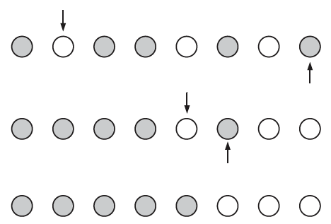
Of course, in the context of implementing the algorithm with code, we need some way of automating the finding of the leftmost white checker and the rightmost red checker — we do that using two pointers. The solution above can be slightly modified to more closely align with the verbiage of the Polish National Flag Problem:
class Solution:
def sortArrayByParity(self, nums: List[int]) -> List[int]:
left = 0
right = len(nums) - 1
# RED is 0 to denote even numbers (zero remainder when divided by 2)
# WHITE is 1 to denote odd numbers (remainder of 1 when divided by 2)
RED = 0
WHITE = 1
while left <= right:
# stop pointing at red checkers until leftmost white checker is encountered
if nums[left] % 2 == RED:
left += 1
# stop pointing at white checkers until rightmost red checker is encountered
elif nums[right] % 2 == WHITE:
right -= 1
# swap the misplaced white (left pointed) and red checkers (right pointed)
else:
nums[left], nums[right] = nums[right], nums[left]
left += 1
right -= 1
return nums
LC 167. Two Sum II - Input Array Is Sorted (✠)
Given an array of integers numbers that is already sorted in ascending order, find two numbers such that they add up to a specific target number.
Return the indices of the two numbers (1-indexed) as an integer array answer of size 2, where 1 <= answer[0] < answer[1] <= numbers.length.
You may assume that each input would have exactly one solution and you may not use the same element twice.
class Solution:
def twoSum(self, numbers: List[int], target: int) -> List[int]:
left = 0
right = len(numbers) - 1
while left < right:
curr = numbers[left] + numbers[right]
if curr < target:
left += 1
elif curr > target:
right -= 1
else:
break
return [left + 1, right + 1]
LC 15. 3Sum (✠)
Given an array nums of n integers, are there elements a, b, c in nums such that a + b + c = 0? Find all unique triplets in the array which gives the sum of zero.
Notice that the solution set must not contain duplicate triplets.
class Solution:
def threeSum(self, nums: List[int]) -> List[List[int]]:
n = len(nums)
nums.sort()
res = []
for i in range(n - 2):
curr = nums[i]
if curr > 0:
break
# skip repeated values to avoid duplicate results
if i > 0 and nums[i-1] == curr:
continue
target = -curr
left = i + 1
right = n - 1
while left < right:
curr_pair = nums[left] + nums[right]
if curr_pair < target:
left += 1
elif curr_pair > target:
right -= 1
else:
res.append([curr, nums[left], nums[right]])
left += 1
right -= 1
# skip the values we just added to avoid duplicate results
while left < right and nums[left] == nums[left - 1]:
left += 1
return res
The two pointers approach for this problem is not obvious, largely because the first step in the two pointers solution is a pre-sorting one (i.e., we sort the array first in order to effectively employ two pointers). Further, we use the "opposite ends" two pointers approach for each iteration through the sorted nums array. Once a two pointer approach is settled on (there are other approaches), the hardest part of the problem is ensuring duplicate results are not included. How this works exactly is best understood by means of an example input (assume the pre-sorting has been done in advance):
nums = [-1, -1, 0, 0, 0, 0, 1, 1, 1]
Before analyzing what happens with the code, let's first identify the desired output (i.e., distinct triples) for this example input, namely the following:
[[-1, 0, 1], [0, 0, 0]]
How does the solution above work to give us this? Let l and r denote the left and right pointers, respectively. And let A denote the current i-value for the iteration and B the end value (third to last). Then we have the following consequences for the first iteration:
A B
[-1, -1, 0, 0, 0, 0, 1, 1, 1]
l r # -1 + (-1 + 1) < 0; increment l
l r # -1 + (0 + 1) == 0; triple: [-1, 0, 1]
l r # increment l, decrement r
l r # increment l (second skip condition)
l r # increment l (second skip condition)
l r # -1 + (1 + 1) > 0; decrement r
l/r # while loop does not execute
And the second iteration:
A B
[-1, -1, 0, 0, 0, 0, 1, 1, 1] # (first skip condition)
Note how the first skip condition ensures we do not create duplicates. If we had continued with the second iteration as shown above, then we would have the following (resulting in a duplicated triple):
A B
[-1, -1, 0, 0, 0, 0, 1, 1, 1]
l r # -1 + (0 + 1) == 0; triple: [-1, 0 ,1]
Now for the third iteration:
A B
[-1, -1, 0, 0, 0, 0, 1, 1, 1]
l r # 0 + (0 + 1) > 0; decrement r
l r # 0 + (0 + 1) > 0; decrement r
l r # 0 + (0 + 1) > 0; decrement r
l r # 0 + (0 + 0) == 0; triple: [0, 0, 0]
l/r # increment l, decrement r
# while loop does not execute
Fourth iteration:
A B
[-1, -1, 0, 0, 0, 0, 1, 1, 1] # (first skip condition)
Fifth iteration:
A B
[-1, -1, 0, 0, 0, 0, 1, 1, 1] # (first skip condition)
Sixth iteration:
A B
[-1, -1, 0, 0, 0, 0, 1, 1, 1] # (first skip condition)
Seventh iteration:
A/B
[-1, -1, 0, 0, 0, 0, 1, 1, 1] # (curr > 0 skip condition)
LC 557. Reverse Words in a String III (✓)
Given a string s, reverse the order of characters in each word within a sentence while still preserving whitespace and initial word order.
class Solution:
def reverseWords(self, s: str) -> str:
def reverseWord(start, end):
while start < end:
res[start], res[end] = res[end], res[start]
start += 1
end -= 1
n = len(s)
res = list(s)
word_start = 0
for i in range(n):
if s[i] == ' ':
reverseWord(word_start, i - 1)
word_start = i + 1
reverseWord(word_start, n - 1)
return ''.join(res)
The directive is simple: reverse each space-separated block of characters (i.e., "word") while leaving the spaces in place. But implementing a solution is perhaps a little trickier than it seems at first.
We can use two pointers on opposite ends for each block of characters, but we need some way of determining where the beginning of each word occurs. The first word will naturally start at index 0 and each subsequent word will start at whatever character occurs first after a space. The end of a word will aways be whatever character was most recently encountered before a space.
LC 917. Reverse Only Letters (✓)
Given a string S, return the "reversed" string where all characters that are not a letter stay in the same place, and all letters reverse their positions.
class Solution:
def reverseOnlyLetters(self, s: str) -> str:
def is_letter(char):
return 65 <= ord(char) <= 90 or 97 <= ord(char) <= 122
left = 0
right = len(s) - 1
res = list(s)
while left < right:
left_is_letter = is_letter(s[left])
right_is_letter = is_letter(s[right])
if not left_is_letter:
left += 1
elif not right_is_letter:
right -= 1
else:
res[left], res[right] = res[right], res[left]
left += 1
right -=1
return ''.join(res)
Note that the use of the is_letter function is highly optimized for this problem because it only considers the ASCII values of lower and uppercase English letters. We could have used Python's str.isalpha() instead, but the extra overhead isn't worth it because it considers letters in all kinds of languages.
LC 2000. Reverse Prefix of Word (✓)
Given a 0-indexed string word and a character ch, reverse the segment of word that starts at index 0 and ends at the index of the first occurrence of ch (inclusive). If the character ch does not exist in word, do nothing.
- For example, if
word = "abcdefd"andch = "d", then you should reverse the segment that starts at0and ends at3(inclusive). The resulting string will be"dcbaefd".
Return the resulting string.
class Solution:
def reversePrefix(self, word: str, ch: str) -> str:
def reverse_chars(end):
start = 0
while start < end:
res[start], res[end] = res[end], res[start]
start += 1
end -= 1
res = list(word)
for i in range(len(res)):
if word[i] == ch:
reverse_chars(i)
return ''.join(res)
return word
LC 75. Sort Colors (✠) ★★
Given an array nums with n objects colored red, white, or blue, sort them in-place so that objects of the same color are adjacent, with the colors in the order red, white, and blue.
We will use the integers 0, 1, and 2 to represent the color red, white, and blue, respectively.
class Solution:
def sortColors(self, nums: List[int]) -> None:
"""
Do not return anything, modify nums in-place instead.
"""
RED = 0
WHITE = 1
BLUE = 2
first_white_pos = 0
left = 0
right = len(nums) - 1
while left <= right:
if nums[left] == RED:
nums[first_white_pos], nums[left] = nums[left], nums[first_white_pos]
left += 1
first_white_pos += 1
elif nums[left] == WHITE:
left += 1
else:
nums[right], nums[left] = nums[left], nums[right]
right -= 1
This problem, which may be considered a more advanced version of LC 905. Sort Array By Parity (i.e., the Polish National Flag Problem due to the Polish flag having colors red and white), is known as the Dutch National Flag Problem (due to the Dutch flag having colors red, white, and blue).
A wonderful framing for this problem appears in [2] (the algorithm's verbal solution also follows from this resource):
There is a row of checkers of three colors: red, white, and blue. Devise an algorithm to rearrange the checkers so that all the red checkers come first, all the white ones come next, and all the blue checkers come last. The only operations allowed are examination of a checker's color and swap of two checkers. Try to minimize the number of swaps made by your algorithm.
The "swap of two checkers" phrase may indicate a two pointers approach could be appropriate. The following algorithm, which can be used with some creativity when implementing the Quicksort sorting algorithm, is based on considering the checker row as made up of four contiguous possibly empty sections: red checkers on the left, then white checkers, then the checkers whose colors are yet to be identified, and finally blue checkers:

Initially, the red, white, and blue sections are empty, with all the checkers being in the unknown section. On each iteration, the algorithm shrinks the size of the unknown section by one element either from the left or from the right: If the first (i.e., leftmost) checker in the unknown section is red, swap it with the first checker after the red section and advance to the next checker; if it is white, advance to the next checker; if it is blue, swap it with the last checker before the blue section. This step is repeated as long as there are checkers in the unknown section.
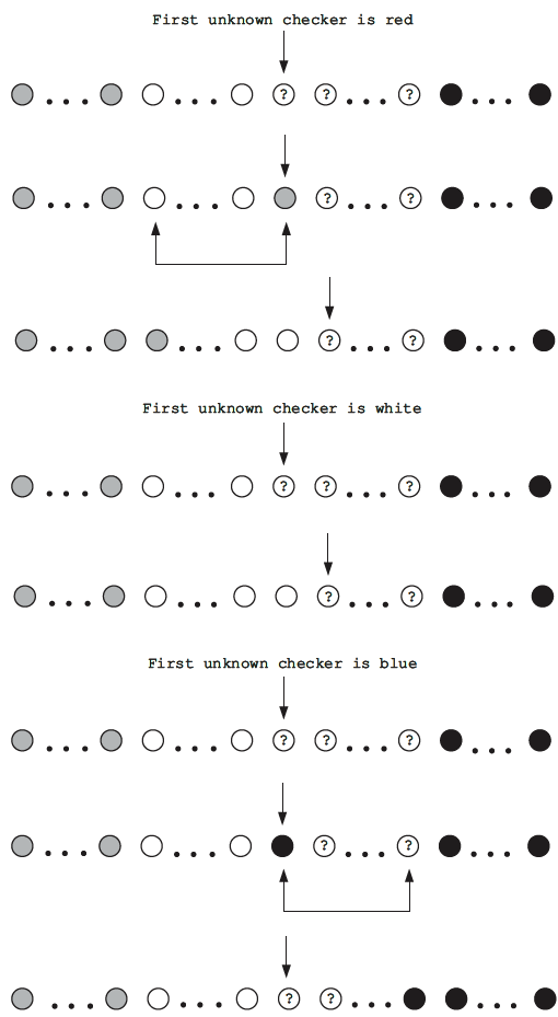
As with LC 905. Sort Array By Parity, however, to actually implement the algorithm illustrated above with code means we're going to need some pointers to keep track of things. The use of two pointers in LC 905 was somewhat straightforward:
class Solution:
def sortArrayByParity(self, nums: List[int]) -> List[int]:
left = 0
right = len(nums) - 1
# RED is 0 to denote even numbers (zero remainder when divided by 2)
# WHITE is 1 to denote odd numbers (remainder of 1 when divided by 2)
RED = 0
WHITE = 1
while left <= right:
# stop pointing at red checkers until leftmost white checker is encountered
if nums[left] % 2 == RED:
left += 1
# stop pointing at white checkers until rightmost red checker is encountered
elif nums[right] % 2 == WHITE:
right -= 1
# swap the misplaced white (left pointed) and red checkers (right pointed)
else:
nums[left], nums[right] = nums[right], nums[left]
left += 1
right -= 1
return nums
We will still use two pointers, left and right, to keep track of the left and right boundaries of the "unknown" zone, pictured previously. But the following part of our algorithm necessitates the addition of another kind of pointer: "If the leftmost checker in the unknown section is red, then swap it with the first checker after the red section (i.e., the first or leftmost white checker) and advance to the next checker." So we basically need three pointers: two for the "unknown" zone (left and right), which shrinks inward as we process checkers, and one for where the first white checker is or should be (first_white_pos).
As long as a white checker is present, the final value of first_white_pos will always point to where the first white checker is. If we print the final nums array as well as the final first_white_pos value, then we'll have the following:
[2,0,2,1,1,0] # initial colors array
[0,0,1,1,2,2] # sorted colors array
2 # first_white_pos final value
If, however, a white checker is not present, then first_white_pos, will point to where the first white checker should be if one were added:
[2,0,2,0,0,0] # initial colors array
[0,0,0,0,2,2] # sorted colors array
4 # first_white_pos final value
LC 912. Sort an Array (✠) ★★
Given an array of integers nums, sort the array in ascending order.
class Solution:
def partition(self, arr, l, r, pivot):
first_pivot = l
while l <= r:
if arr[l] < pivot:
arr[first_pivot], arr[l] = arr[l], arr[first_pivot]
l += 1
first_pivot += 1
elif arr[l] == pivot:
l += 1
else:
arr[r], arr[l] = arr[l], arr[r]
r -= 1
return first_pivot, r
def qsort_inplace(self, arr, left, right):
if left >= right:
return
pivot = arr[random.randint(left, right)]
pivot_start, pivot_end = self.partition(arr, left, right, pivot)
self.qsort_inplace(arr, left, pivot_start - 1)
self.qsort_inplace(arr, pivot_end + 1, right)
def sortArray(self, nums: List[int]) -> List[int]:
self.qsort_inplace(nums, 0, len(nums) - 1)
return nums
The official solution provides illustrative implementations of the following sorting algorithms: merge sort, heap sort, counting sort, and radix sort. The sort above, quick sort, is really meant to illustrate how a well-known and often used sorting algorithm (qucksort) fundamentally uses a two pointer strategy behind the scenes for one of its most efficient implementations (i.e., the in-place manipulation of its elements). The partition method of the code block above serves to highlight where the two pointer strategy is being used.
This strategy is effectively the same as that used in LC 75. Sort Colors. The discussion below details the differences more clearly.
Compare the solutions to LC 75 and LC 912 side by side (the two pointer similarities are highlighted):
class Solution:
def partition(self, arr, l, r, pivot):
first_pivot = l
while l <= r:
if arr[l] < pivot:
arr[first_pivot], arr[l] = arr[l], arr[first_pivot]
l += 1
first_pivot += 1
elif arr[l] == pivot:
l += 1
else:
arr[r], arr[l] = arr[l], arr[r]
r -= 1
return first_pivot, r
def qsort_inplace(self, arr, left, right):
if left >= right:
return
pivot = arr[random.randint(left, right)]
pivot_start, pivot_end = self.partition(arr, left, right, pivot)
self.qsort_inplace(arr, left, pivot_start - 1)
self.qsort_inplace(arr, pivot_end + 1, right)
def sortArray(self, nums: List[int]) -> List[int]:
self.qsort_inplace(nums, 0, len(nums) - 1)
return nums
class Solution:
def sortColors(self, nums: List[int]) -> None:
"""
Do not return anything, modify nums in-place instead.
"""
RED = 0
WHITE = 1
BLUE = 2
first_white_pos = 0
left = 0
right = len(nums) - 1
while left <= right:
if nums[left] == RED:
nums[first_white_pos], nums[left] = nums[left], nums[first_white_pos]
left += 1
first_white_pos += 1
elif nums[left] == WHITE:
left += 1
else:
nums[right], nums[left] = nums[left], nums[right]
right -= 1
How is the partition method of in-place quicksort (left) similar to the Dutch flag problem solution (right)? They're very similar! Almost the same. For the Dutch flag problem, the values 0, 1, and 2 represented RED, WHITE, and BLUE, respectively. For in-place quicksort, values smaller than the pivot represent RED, values equal to the pivot represent WHITE, and values greater than the pivot represent BLUE.
We still fundamentally start with the following overall situation:
The difference for this sorting problem that makes it somewhat more complicated than the Dutch flag problem is that we recursively solve smaller and smaller instances of the same subproblem (as opposed to sorting all values in a single pass).
For example, suppose nums = [3,7,4,10,8,1,3,4,3,2] is our original array and that the random pivot we get is the index value of 6, meaning nums[6] = 3 serves as our pivot. Then the initial partition method will result in something similar to the following array of numbers (i.e., where all numbers have been partitioned in such a way that every number less than the pivot lies to the left while every number greater than the pivot lies to the right):
[2,1,3,3,3,8,4,10,4,7]
The genius of quicksort is that each value of 3, after the first partition, is where it should permanently belong for the final sorted array. Our original problem of sorting nums = [3,7,4,10,8,1,3,4,3,2] has now been reduced to the following smaller instances of the same problem:
[3,7,4,10,8,1,3,4,3,2] # initial array; pivot -> nums[6] = 3
[2,1,3,3,3,8,4,10,4,7] # result after first partition
[2,1] [8,4,10,4,7] # subproblems to be solved
Exhaust inputs
Remarks
Sometimes a problem provides two or more iterables as input. In such cases, specifically with two iterables (e.g., arrays), we can move pointers along both inputs simultaneously until all elements have been checked or exhausted. The idea is to have logic that uses both inputs (or more in some cases) in some fashion until one of them has been exhausted. Then logic is passed on so the other input is similarly exhausted.
This approach generally has a linear time complexity of , where and represent the lengths of the first and second iterables, respectively. Why? Because at every iteration we move at least one pointer forward, meaning the pointers cannot be moved forward more than times without the iterables being exhausted.
def fn(arr1, arr2):
i = j = 0
while i < len(arr1) and j < len(arr2):
# choose one of the following depending on the problem:
# i += 1
# j += 1
# increment i AND j: i+= 1 and j += 1
while i < len(arr1):
i += 1
while j < len(arr2):
j += 1
Examples
Merge two sorted arrays into another sorted array (✓)
def merge_sorted_arrs(arr1, arr2):
i = j = 0
res = []
while i < len(arr1) and j < len(arr2):
if arr1[i] < arr2[j]:
res.append(arr1[i])
i += 1
elif arr1[i] > arr2[j]:
res.append(arr2[j])
j += 1
else:
res.append(arr1[i])
res.append(arr2[j])
i += 1
j += 1
while i < len(arr1):
res.append(arr1[i])
i += 1
while j < len(arr2):
res.append(arr2[j])
j += 1
return res
Time: . The time complexity here is , where n == len(arr1) and m == len(arr2), because we never make more than iterations. We gradually process both arrays completely, and the work done within each while loop along the way is .
Space: . The space complexity here is because we do not typically include the output we're building towards the space complexity computation itself; nonetheless, one could make the argument the space complexity is also because we end up creating an array that we return with elements.
LC 350. Intersection of Two Arrays II (✠)
Given two integer arrays nums1 and nums2, return an array of their intersection. Each element in the result must appear as many times as it shows in both arrays and you may return the result in any order.
class Solution:
def intersect(self, nums1: List[int], nums2: List[int]) -> List[int]:
nums1.sort()
nums2.sort()
res = []
p1 = p2 = 0
while p1 < len(nums1) and p2 < len(nums2):
if nums1[p1] == nums2[p2]:
res.append(nums1[p1])
p1 += 1
p2 += 1
elif nums1[p1] > nums2[p2]:
p2 += 1
else:
p1 += 1
return res
Pre-sorting is a common theme for employing two pointer solutions.
LC 349. Intersection of Two Arrays (✠)
Given two integer arrays nums1 and nums2, return an array of their intersection. Each element in the result must be unique and you may return the result in any order.
class Solution:
def intersection(self, nums1: List[int], nums2: List[int]) -> List[int]:
nums1.sort()
nums2.sort()
res = []
p1 = p2 = 0
while p1 < len(nums1) and p2 < len(nums2):
if nums1[p1] == nums2[p2]:
if len(res) == 0 or res[-1] != nums1[p1]:
res.append(nums1[p1])
p1 += 1
p2 += 1
elif nums1[p1] > nums2[p2]:
p2 += 1
else:
p1 += 1
return res
The solution above is equivalent to that for LC 350. Intersection of Two Arrays II, where the only difference is the addition of the following conditional to prevent duplicates:
if len(res) == 0 or res[-1] != nums1[p1]:
res.append(nums1[p1])
A more optimal solution might be to use sets since lookup time is :
def intersection(nums1, nums2):
set1, set2 = set(nums1), set(nums2)
return [x for x in set1 if x in set2]
LC 986. Interval List Intersections (✠)
You are given two lists of closed intervals, firstList and secondList, where firstList[i] = [starti, endi] and secondList[j] = [startj, endj]. Each list of intervals is pairwise disjoint and in sorted order.
Return the intersection of these two interval lists.
A closed interval [a, b] (with a < b) denotes the set of real numbers x with a <= x <= b.
The intersection of two closed intervals is a set of real numbers that are either empty or represented as a closed interval. For example, the intersection of [1, 3] and [2, 4] is [2, 3].
class Solution:
def intervalIntersection(self, firstList: List[List[int]], secondList: List[List[int]]) -> List[List[int]]:
res = []
p1 = p2 = 0
while p1 < len(firstList) and p2 < len(secondList):
f_start = firstList[p1][0]
f_end = firstList[p1][1]
s_start = secondList[p2][0]
s_end = secondList[p2][1]
# determine if firstList[p1] intersects secondList[p2]
lo = max(f_start, s_start)
hi = min(f_end, s_end)
if lo <= hi:
res.append([lo, hi])
# remove interval with smallest endpoint
if f_end < s_end:
p1 += 1
else:
p2 += 1
return res
The two pointer approach above is probably the cleanest implementation for this problem. The strategy is deceptively simple: determine whether or not the linked intervals overlap (if so, add the intersection to the results array) and then increment past whichever interval has the smallest endpoint.
We do not have to worry about missing any intersected intervals in the last conditional of the while loop (i.e., the removal of the interval with the smallest endpoint) because of the condition that the intervals in each list are pairwise disjoint. That is, for whichever while loop iteration we are currently processing, the interval with the smallest endpoint can only intersect a single interval in the other list (otherwise, the other list would have to have overlapping intervals, which violates the pairwise disjoint condition).
Another less polished two pointer solution might be the following, but it just overcomplicates things:
class Solution:
def intervalIntersection(self, firstList: List[List[int]], secondList: List[List[int]]) -> List[List[int]]:
res = []
p1 = p2 = 0
while p1 < len(firstList) and p2 < len(secondList):
f_start = firstList[p1][0]
f_end = firstList[p1][1]
s_start = secondList[p2][0]
s_end = secondList[p2][1]
if f_end < s_start:
p1 += 1
elif s_end < f_start:
p2 += 1
else:
res.append([max(f_start, s_start), min(f_end, s_end)])
if f_end > s_end:
p2 += 1
else:
p1 += 1
return res
LC 2540. Minimum Common Value (✓)
Given two integer arrays nums1 and nums2, sorted in non-decreasing order, return the minimum integer common to both arrays. If there is no common integer amongst nums1 and nums2, return -1.
Note that an integer is said to be common to nums1 and nums2 if both arrays have at least one occurrence of that integer.
class Solution:
def getCommon(self, nums1: List[int], nums2: List[int]) -> int:
i = j = 0
while i < len(nums1) and j < len(nums2):
if nums1[i] < nums2[j]:
i += 1
elif nums2[j] < nums1[i]:
j += 1
else:
return nums1[i]
return -1
The idea here is that we keep advancing one pointer until it overshoots the value referenced by the other pointer. Then we switch pointers and do the same. This will eventually leads us to the first common value or we'll exhaust both inputs and return -1, indicating there is no common element, as desired.
LC 844. Backspace String Compare (✓) ★★★
Given two strings s and t, return true if they are equal when both are typed into empty text editors. '#' means a backspace character.
Note that after backspacing an empty text, the text will continue empty.
class Solution:
def backspaceCompare(self, s: str, t: str) -> bool:
def next_valid_char(r, start_pos):
skip = 0
for i in range(start_pos, -1, -1):
if r[i] == '#':
skip += 1
elif skip > 0:
skip -= 1
else:
return i
return -1
s_p = len(s) - 1
t_p = len(t) - 1
# still characters to process
while s_p >= 0 or t_p >= 0:
s_p = next_valid_char(s, s_p)
t_p = next_valid_char(t, t_p)
# both strings are fully processed
if s_p < 0 and t_p < 0:
return True
# one string is not fully processed but the other one is
# OR the current valid characters don't match
elif (s_p < 0 or t_p < 0) or s[s_p] != t[t_p]:
return False
# a match is made for the valid characters so we continue
else:
s_p -= 1
t_p -= 1
return True
This is not a typical "exhaust both inputs" two pointer problem. The stack-based solution is somewhat clear from the outset:
class Solution:
def backspaceCompare(self, s: str, t: str) -> bool:
def get_str(r):
stack = []
for char in r:
if char == '#':
if stack:
stack.pop()
else:
stack.append(char)
return "".join(stack)
s_str = get_str(s)
t_str = get_str(t)
return s_str == t_str
But this is time and space, but as the follow-up for this problem suggests, we can do better on the space, specifically . And we use two pointers to accomplish that.
The key observation is to consider both strings from their ends. We only ever want to compare characters we know to be valid for the eventual final string. Iterating from the front is a non-starter since we don't know in advance how many backspace characters # we'll encounter. But if we iterate from the back, then we can treat # characters as skips and track their count. The next_valid_char utility function lets us look at each string to determine what their next valid characters at the end would be, returning the valid character's position or -1 if no next valid character is available.
We then take the return values from next_valid_char and perform some logic to determine whether or not we should keep processing the strings:
- If all we did was skip through the rest of all the characters for both strings, then clearly the strings must be equal.
- If we skipped through everything in one string but still have characters remaining in the other string, then these strings couldn't possibly be equal. Additionally, if we have valid characters from both strings but they're not equal, then again the strings have to be unequal.
- Finally, if both checks above don't flag the processing as completed, then we need to continue on by advancing to the next character.
We can actually generalize the logic in the next_valid_char function to handle iterables of any kind where skip conditions are made and we want the rightmost valid element:
def next_valid_element(arr_or_str, start_pos):
# declare elements for which skips will be made
one_skip_elements = { '#', '!' }
two_skip_elements = { '@', '%', '*' }
three_skip_elements = { '^' }
# always start with 0 skips
skip = 0
# process entire iterable until valid element is found
for i in range(start_pos, -1, -1):
el = arr_or_str[i]
# one or more skips needed
if el in one_skip_elements:
skip += 1
elif el in two_skip_elements:
skip += 2
elif el in three_skip_elements:
skip += 3
# valid element found but skips exist
elif skip > 0:
skip -= 1
# valid element found and no skips: return position
else:
return i
# no valid element was found
return -1
Fast and slow
Remarks
The "fast and slow" template provided below is not for problems involving linked lists but for other commonly encountered problems where the iterable given is an array, string (array of characters), etc. The idea is that the fast pointer steadily advances while the slow pointer is only advanced in a piecemeal fashion (often after some sort of condition is met).
def fn(arr):
slow = fast = 0
while fast < len(arr):
if CONDITION:
slow += 1
fast += 1
return slow
Examples
LC 392. Is Subsequence (✓)
Given two strings s and t, check if s is a subsequence of t.
A subsequence of a string is a new string that is formed from the original string by deleting some (can be none) of the characters without disturbing the relative positions of the remaining characters. (i.e., "ace" is a subsequence of "abcde" while "aec" is not).
class Solution:
def isSubsequence(self, s: str, t: str) -> bool:
# not possible for s to be a subsequence of t (micro-optimization)
if len(s) > len(t):
return False
# s must be a subsequence of t if s is empty
if len(s) == 0:
return True
slow = fast = 0
while fast < len(t):
if s[slow] == t[fast]:
slow += 1
if slow == len(s):
return True
fast += 1
return False
Note that the condition if len(s) == 0: return True is not just a micro-optimization in the solution above since we return False at the end (due to always checking for an early return with if slow == len(s): return True).
Time: . If n == len(t), then there is a chance we could end up iterating through all of the characters in t, but that is the worst-case scenario.
Space: . There is only a constant amount of space used to solve this problem.
LC 26. Remove Duplicates from Sorted Array (✠)
Given an integer array nums sorted in non-decreasing order, remove the duplicates in-place such that each unique element appears only once. The relative order of the elements should be kept the same.
Since it is impossible to change the length of the array in some languages, you must instead have the result be placed in the first part of the array nums. More formally, if there are k elements after removing the duplicates, then the first k elements of nums should hold the final result. It does not matter what you leave beyond the first k elements.
Return k after placing the final result in the first k slots of nums.
Do not allocate extra space for another array. You must do this by modifying the input array in-place with extra memory.
Custom Judge:
The judge will test your solution with the following code:
int[] nums = [...]; // Input array
int[] expectedNums = [...]; // The expected answer with correct length
int k = removeDuplicates(nums); // Calls your implementation
assert k == expectedNums.length;
for (int i = 0; i < k; i++) {
assert nums[i] == expectedNums[i];
}
If all assertions pass, then your solution will be accepted.
class Solution:
def removeDuplicates(self, nums: List[int]) -> int:
slow = fast = 1
while fast < len(nums):
if nums[fast] != nums[fast-1]:
nums[slow] = nums[fast]
slow += 1
fast += 1
return slow
The first number cannot be a duplicate; hence, we start both pointers at index 1. The idea, then, is that we progressively overwrite the contents of nums using the slow pointer once a yet-unencountered number is reached (we're gauranteed to encounter only new numbers since the input array is sorted).
Given how this specific problem is set up, the following solution may be considered slightly cleaner than the one above:
class Solution:
def removeDuplicates(self, nums: List[int]) -> int:
slow = 1
for fast in range(1, len(nums)):
if nums[fast] != nums[fast-1]:
nums[slow] = nums[fast]
slow += 1
return slow
LC 27. Remove Element (✠)
Given an integer array nums and an integer val, remove all occurrences of val in nums in-place. The relative order of the elements may be changed.
Since it is impossible to change the length of the array in some languages, you must instead have the result be placed in the first part of the array nums. More formally, if there are k elements after removing the duplicates, then the first k elements of nums should hold the final result. It does not matter what you leave beyond the first k elements.
Return k after placing the final result in the first k slots of nums.
Do not allocate extra space for another array. You must do this by modifying the input array in-place with extra memory.
Custom Judge:
The judge will test your solution with the following code:
int[] nums = [...]; // Input array
int val = ...; // Value to remove
int[] expectedNums = [...]; // The expected answer with correct length.
// It is sorted with no values equaling val.
int k = removeElement(nums, val); // Calls your implementation
assert k == expectedNums.length;
sort(nums, 0, k); // Sort the first k elements of nums
for (int i = 0; i < actualLength; i++) {
assert nums[i] == expectedNums[i];
}
If all assertions pass, then your solution will be accepted.
class Solution:
def removeElement(self, nums: List[int], val: int) -> int:
slow = fast = 0
while fast < len(nums):
if nums[fast] != val:
nums[slow] = nums[fast]
slow += 1
fast += 1
return slow
The two pointer solution here is arguably a bit of a mind-bender at first, but it becomes quite clear after some reflection. The basic idea: move the slow pointer continuously until it hits the first val that needs to be removed. Then, whenever the fast pointer encounters an element not equal to val, swap the elements that slow and fast point to (val and non-val elements, respectively). Wherever slow ends up pointing (in terms of index value) is the final length of the array whose elements have not been removed.
To see the logic unfold, try moving along the i and j pointers below (representing the slow and fast pointers, respectively) and swapping values as the solution logic requires:
val = 2
[0,1,2,2,3,0,4,2]
i
j
For example, i and j move together until the first 2 is reached:
[0,1,2,2,3,0,4,2]
i
j
And then j continues forward until the 3 is encountered:
[0,1,2,2,3,0,4,2]
i
j
At this point, we swap the elements that i and j point to and then increment i:
[0,1,3,2,2,0,4,2]
i
j
And we continue along until the input array nums has been exhausted by j. Where i last points in terms of index value will be the length of the array without val present.
Given the structure of this problem, it's common to see a solution also represented as follows:
class Solution:
def removeElement(self, nums: List[int], val: int) -> int:
i = 0
for j in range(len(nums)):
if nums[j] != val:
nums[i] = nums[j]
i += 1
return i
LC 283. Move Zeroes (✓, ✠)
Given an integer array nums, move all 0's to the end of it while maintaining the relative order of the non-zero elements.
Note that you must do this in-place without making a copy of the array.
class Solution:
def moveZeroes(self, nums: List[int]) -> None:
"""
Do not return anything, modify nums in-place instead.
"""
slow = fast = 0
while fast < len(nums):
if nums[fast] != 0:
nums[slow], nums[fast] = nums[fast], nums[slow]
slow += 1
fast += 1
The idea is for the slow pointer to always point to a 0 value and to wait until the fast pointer encounters a non-0 value so that a swap can be made (and then slow incremented). For example, we could have a start like the following (i and j represent the slow and fast pointers, respectively):
[1,0,0,3,12]
i
j
The first value is not 0 so a vacuous swap occurs and both pointers are incremented:
[1,0,0,3,12]
i
j
Then j is incremented again to 0. Then again to 3, which is where a swap will need to occur:
[1,0,0,3,12]
i
j
Once the swap occurs and i is incremented, we have the following:
[1,3,0,0,12]
i
j
It should be clear now how the relative ordering is respected, all while pushing the 0 values to the end of the array.
Miscellaneous
Build a trie
Remarks
TBD
TBD
Examples
TBD
Hashing (and sets)
Checking for existence
Remarks
This is where hash maps (and sets) really shine. Checking whether or not an element exists in a hash table is an operation. Checking for existence in an array, however, is an operation. This means a number of algorithms can often be improved from to by using a hash map instead of an array to check for existence.
lookup = {}
if key in lookup: # existence check is O(1) for hash maps
# ...
seen = set()
if el in seen: # existence check is O(1) for sets
# ...
Examples
LC 1. Two Sum (✓)
Given an array of integers nums and an integer target, return indices of the two numbers such that they add up to target.
You may assume that each input would have exactly one solution, and you may not use the same element twice.
You can return the answer in any order.
class Solution:
def twoSum(self, nums: List[int], target: int) -> List[int]:
lookup = {}
for i in range(len(nums)):
complement = target - nums[i]
if complement in lookup:
return [lookup[complement], i]
lookup[nums[i]] = i
The key insight for solving this classic problem involves recognizing that the lookup time in hash maps can be used to great effect here. Quickly determining whether or not the complement for a given number exists in the lookup hash map makes it possible for the overall time complexity to be and not .
Time: . We make a single pass in time where n == len(nums).
Space: . It takes space to build the lookup hash map itself.
LC 2351. First Letter to Appear Twice (✓)
Given a string s consisting of lowercase English letters, return the first letter to appear twice.
Note:
- A letter
aappears twice before another letterbif the second occurrence ofais before the second occurrence ofb. swill contain at least one letter that appears twice.
class Solution:
def repeatedCharacter(self, s: str) -> str:
lookup = set()
for char in s:
if char in lookup:
return char
lookup.add(char)
The efficiency of the solution above completely relies on the fact that lookups in sets are .
Time: . We iterate through all characters in s, meaning the overall time complexity is , where n == len(s).
Space: . Building the seen lookup set appears to consume extra memory, but the reality is that seen hold at most 26 characters since s is comprised of only lowercase English letters. Hence, the space is really . But if we don't know the exact character set, then it would be clearer to say the solution above has space complexity or where represents the total number of characters in the character set being considered.
Determining unique numbers based on non-existent off-by-ones (✓)
Given an integer array nums, find all the unique numbers x in nums that satisfy the following: x + 1 is not in nums, and x - 1 is not in nums.
def find_numbers(nums):
lookup = set(nums)
res = []
for num in lookup:
if (num + 1 not in lookup) and (num - 1 not in lookup):
res.append(num)
return res
First convert nums to a set in order to avoid considering non-unique elements. Then process each unique element to see whether or not its "off-by-one" neighbors exist.
Time: . It takes time to build the lookup set and time to process each number, resulting in an overall time complexity of .
Space: . We consume additional memory by building the lookup set.
LC 1832. Check if the Sentence Is Pangram (✓)
A pangram is a sentence where every letter of the English alphabet appears at least once.
Given a string sentence containing only lowercase English letters, return true if sentence is a pangram, or false otherwise.
class Solution:
def checkIfPangram(self, sentence: str) -> bool:
seen = set()
for char in sentence:
seen.add(char)
if len(seen) == 26:
return True
return False
The solution above is methodical and does not rely on the built-in set command, but we could just as well:
class Solution:
def checkIfPangram(self, sentence: str) -> bool:
return len(set(sentence)) == 26
The time and space complexity are the same for both approaches.
Time: . We process each character of sentence, where n == len(sentence).
Space: . Constructing the set in either solution scales with the input size. Since we're limited to lowercase English letters, we technically have a constant space complexity, but it may be more accurate to say , where represents the size of the character set(s) that may be valid to use.
LC 268. Missing Number (✓)
Given an array nums containing n distinct numbers in the range [0, n], return the only number in the range that is missing from the array.
Follow up: Could you implement a solution using only O(1) extra space complexity and O(n) runtime complexity?
class Solution:
def missingNumber(self, nums):
lookup = set(nums)
n = len(nums)
for num in range(n + 1):
if num not in lookup:
return num
The approach above is likely the intended solution. Using lookups means our overall time complexity will be .
Time: . We iterate over numbers in total, meaning our overall time complexity is .
Space: . Building the lookup set consumes additional memory.
Just because we can solve this problem using a hash map does not mean we should. There are two solutions that are notably better, and they both rely on basic mathematical observations.
Using Gauss's formula (sum of first positive integers):
class Solution:
def missingNumber(self, nums: List[int]) -> int:
n = len(nums)
target_sum = n * (n + 1) // 2
actual_sum = sum(nums)
return target_sum - actual_sum
Another effective mathematical approach involves computing a running sum of the first positive integers — the difference is the missing number:
class Solution:
def missingNumber(self, nums: List[int]) -> int:
running_sum = 0
for i in range(len(nums)):
running_sum += (i + 1) - nums[i]
return running_sum
Both approaches result in reducing the space complexity from to .
LC 1426. Counting Elements (✓)
Given an integer array arr, count how many elements x there are, such that x + 1 is also in arr. If there are duplicates in arr, count them separately.
class Solution:
def countElements(self, arr: List[int]) -> int:
lookup = set(arr)
res = 0
for num in arr:
if (num + 1) in lookup:
res += 1
return res
The key idea is to use lookup for lookups. Then membership checks for x + 1 for any number x is constant.
Time: . Building the lookup set takes time and subsequently processing each number in arr takes time; hence, overall, the time complexity is .
Space: . The additional space consumed in building the lookup set is .
LC 49. Group Anagrams (✓)
Given an array of strings strs, group the anagrams together. You can return the answer in any order.
An anagram is a word or phrase formed by rearranging the letters of a different word or phrase, typically using all the original letters exactly once.
class Solution:
def groupAnagrams(self, strs: List[str]) -> List[List[str]]:
lookup = defaultdict(list)
for s in strs:
key = "".join(sorted(s))
lookup[key].append(s)
return list(lookup.values())
It's easier to check if a string is an anagram of another string by determining whether or not the sorted versions of these strings are equivalent. To return the groups of anagrams, we add the sorted version of a string as the key in a hash map (for efficient lookups) and we add the string itself to the group if its sorted version matches a key.
Time: . Each string s in strs is processed, where n == len(strs), and k is the length of the longest string in strs.
Space: . n strings must be stored, and the max size of a string is k.
LC 2352. Equal Row and Column Pairs (✓) ★
Given a 0-indexed n x n integer matrix grid, return the number of pairs (Ri, Cj) such that row Ri and column Cj are equal.
A row and column pair is considered equal if they contain the same elements in the same order (i.e. an equal array).
class Solution:
def equalPairs(self, grid: List[List[int]]) -> int:
n = len(grid)
col_lookup = defaultdict(int)
for col in range(n):
column_vals = []
for row in range(n):
column_vals.append(grid[row][col])
col_lookup[tuple(column_vals)] += 1
ans = 0
for row in grid:
ans += col_lookup[tuple(row)]
return ans
This problem is essentially an existence problem. The col_lookup hash map tracks the frequency with which the same sequence of column values appears (separate columns with the same sequence of values must be counted separately). Then we simply need to iterate over all rows and add the number of times the equivalent sequence of values appears for columns. Since hash maps generally need to have immutable keys, we use Python's tuple.
Time: . Each number in the grid is processed.
Space: . The worst case scenario is that each column is unique, meaning col_lookup is of length n, and each member of col_lookup is of length n.
LC 383. Ransom Note (✓)
Given two strings ransomNote and magazine, return true if ransomNote can be constructed by using the letters from magazine and false otherwise.
Each letter in magazine can only be used once in ransomNote.
class Solution:
def canConstruct(self, ransomNote: str, magazine: str) -> bool:
if len(ransomNote) > len(magazine):
return False
lookup = defaultdict(int)
for letter in magazine:
lookup[letter] += 1
for letter in ransomNote:
if lookup[letter] == 0:
return False
lookup[letter] -= 1
return True
The idea is to chip away at ransomNote one character at a time. To do this efficiently, we convert the characters in magazine into a hash map for efficient frequency lookups. If the letter we are trying to chip away from the ransomNote does not exist in the magazine lookup, then we know a solution is not possible.
Time: . We process all characters in ransomNote and magazine, where n == len(magazine).
Space: . We're told all characters are lowercase English, but might be more accurate if we're willing to accommodate more character sets.
LC 217. Contains Duplicate (✓)
Given an integer array nums, return true if any value appears at least twice in the array, and return false if every element is distinct.
class Solution:
def containsDuplicate(self, nums: List[int]) -> bool:
lookup = set()
for num in nums:
if num in lookup:
return True
lookup.add(num)
return False
The solution above is straightforward, but an even more straightforward solution is as follows:
class Solution:
def containsDuplicate(self, nums: List[int]) -> bool:
return len(nums) != len(set(nums))
LC 1436. Destination City (✓)
You are given the array paths, where paths[i] = [cityAi, cityBi] means there exists a direct path going from cityAi to cityBi. Return the destination city, that is, the city without any path outgoing to another city.
It is guaranteed that the graph of paths forms a line without any loop, therefore, there will be exactly one destination city.
class Solution:
def destCity(self, paths: List[List[str]]) -> str:
departures = set()
destinations = set()
for path in paths:
departures.add(path[0])
destinations.add(path[1])
for destination in destinations:
if destination not in departures:
return destination
The solution above explicitly answers the question we are trying to answer: which destination city is not a departure city? Another more Pythonic solution may be expressed as follows:
class Solution:
def destCity(self, paths: List[List[str]]) -> str:
departures, destinations = zip(*paths)
destination_city = set(destinations) - set(departures)
return destination_city.pop()
LC 1496. Path Crossing (✓)
Given a string path, where path[i] = 'N', 'S', 'E' or 'W', each representing moving one unit north, south, east, or west, respectively. You start at the origin (0, 0) on a 2D plane and walk on the path specified by path.
Return True if the path crosses itself at any point, that is, if at any time you are on a location you've previously visited. Return False otherwise.
class Solution:
def isPathCrossing(self, path: str) -> bool:
dirs = {
"N": (0, 1),
"S": (0, -1),
"W": (-1, 0),
"E": (1, 0)
}
seen = {(0, 0)}
x = 0
y = 0
for move in path:
dx, dy = dirs[move]
x += dx
y += dy
if (x, y) in seen:
return True
seen.add((x, y))
return False
LC 205. Isomorphic Strings (✓) ★★
Given two strings s and t, determine if they are isomorphic.
Two strings s and t are isomorphic if the characters in s can be replaced to get t.
All occurrences of a character must be replaced with another character while preserving the order of characters. No two characters may map to the same character, but a character may map to itself.
class Solution:
def isIsomorphic(self, s: str, t: str) -> bool:
s_lookup = defaultdict(list)
t_lookup = defaultdict(list)
for i in range(len(s)):
char_s = s[i]
char_t = t[i]
s_lookup[char_s].append(i)
t_lookup[char_t].append(i)
return sorted(s_lookup.values()) == sorted(t_lookup.values())
The solution above is probably one of the more natural solutions even though it is not the most efficient. The idea is to keep track of the positional values for the different characters in each string — if the sorted lists are the same, then the strings must be isomorphic.
A more efficient way of crafting a solution is to come up with a nifty way of effectively "encoding" each string:
class Solution:
def isIsomorphic(self, s: str, t: str) -> bool:
def encode(s):
lookup = {}
encoding = []
for char in s:
if char not in lookup:
lookup[char] = len(lookup)
encoding.append(lookup[char])
return str(encoding)
return encode(s) == encode(t)
The encode function "encodes" a string by mapping each unique character to a unique integer, based on the order in which the character first appears in the string. It effectively allows us to sidestep the need for direct character comparison, instead relying on the position-based pattern of appearances.
For example, here's how the string "hello" would be encoded:
- For
h, since it's new,lookup[h] = 0. The encoding list begins as[0]. - For
e, since it's new,lookup[e] = 1. The encoding list updates to[0, 1]. - For the first
l, since it's new,lookup[l] = 2. The encoding list updates to[0, 1, 2]. - For the second
l, it's already inlookupwithlookup[l] = 2. The encoding list updates to[0, 1, 2, 2]. - For
o, since it's new,lookup[o] = 3. The encoding list updates to[0, 1, 2, 2, 3].
The final encoded string representation for "hello" is thus "0, 1, 2, 2, 3". As noted on LeetCode, this solution is more modular and allows us to potentially solve interesting follow-up questions like "grouping isomorphic strings":
def groupIsomorphic(strs):
def encode(s):
lookup = {}
encoding = []
for char in s:
if char not in lookup:
lookup[char] = len(lookup)
encoding.append(lookup[char])
return str(encoding)
groups = defaultdict(list)
for s in strs:
encoding = encode(s)
groups[encoding].append(s)
return list(groups.values())
print(groupIsomorphic(['aab', 'xxy', 'xyz', 'abc', 'def', 'xyx']))
"""
[
['aab', 'xxy'],
['xyz', 'abc', 'def'],
['xyx']
]
"""
LC 290. Word Pattern (✓) ★★
Given a pattern and a string s, find if s follows the same pattern.
Here follow means a full match, such that there is a bijection between a letter in pattern and a non-empty word in s.
class Solution:
def wordPattern(self, pattern: str, s: str) -> bool:
def encode(it):
lookup = {}
encoding = []
for el in it:
if el not in lookup:
lookup[el] = len(lookup)
encoding.append(lookup[el])
return str(encoding)
return encode(pattern) == encode(s.split(' '))
This problem is very similar to LC 290. Word Pattern. The efficient solution above exploits the same encoding idea: the items are encoded so as to facilitate positional matching; that is, characters of pattern contribute to the encoding while words of s contribute to the encoding.
LC 791. Custom Sort String (✓)
S and T are strings composed of lowercase letters. In S, no letter occurs more than once.
S was sorted in some custom order previously. We want to permute the characters of T so that they match the order that S was sorted. More specifically, if x occurs before y in S, then x should occur before y in the returned string.
Return any permutation of T (as a string) that satisfies this property.
class Solution:
def customSortString(self, order: str, s: str) -> str:
lookup = defaultdict(int)
for char in s:
lookup[char] += 1
ans = []
for char in order:
if char in lookup:
for _ in range(lookup[char]):
ans.append(char)
del lookup[char]
for char in lookup:
for _ in range(lookup[char]):
ans.append(char)
return "".join(ans)
The idea is to first create a hash map of the character frequencies in s. This will let us recreate a permutation of s efficiently. Now we simply iterate through order from left to right, filling in the ans array with the character counts obtained previously. Lastly, since the order does not matter, we can just fill in the rest of the array with the unused characters and their frequencies.
LC 1657. Determine if Two Strings Are Close (✓) ★
Two strings are considered close if you can attain one from the other using the following operations:
- Operation 1: Swap any two existing characters.
- For example,
abcde -> aecdb
- For example,
- Operation 2: Transform every occurrence of one existing character into another existing character, and do the same with the other character.
- For example,
aacabb -> bbcbaa(alla's turn intob's, and allb's turn intoa's)
- For example,
You can use the operations on either string as many times as necessary.
Given two strings, word1 and word2, return true if word1 and word2 are close, and false otherwise.
class Solution:
def closeStrings(self, word1: str, word2: str) -> bool:
if len(word1) != len(word2):
return False
w1_lookup = defaultdict(int)
w2_lookup = defaultdict(int)
for i in range(len(word1)):
w1_char = word1[i]
w2_char = word2[i]
w1_lookup[w1_char] += 1
w2_lookup[w2_char] += 1
char_match = w1_lookup.keys() == w2_lookup.keys()
freqs_match = sorted(w1_lookup.values()) == sorted(w2_lookup.values())
return char_match and freqs_match
If the words do not have the same length, then nothing can be done to make them equivalent. Since we are only allowed to change one letter into another and not create new letters, the set of unique letters in each word must be identical. Additionally, the list of frequencies needs to be the same to account for single-swaps or all-swaps.
Counting
Remarks
Counting is a very common pattern with hash maps, where "counting" generally refers to tracking the frequency of different elements.
In sliding window problems, a frequent constraint is limiting the amount of a certain element in the window. For example, maybe we're trying to find the longest substring with at most k 0s. In such problems, simply using an integer variable curr is enough to handle the constraint because we are only focused on a single element, namely 0. The template for variable width sliding window problems naturally suggests the use of curr for such situations:
def fn(arr):
left = curr = ans = 0
for right in range(len(arr)):
curr += nums[right]
while left <= right and WINDOW_IS_INVALID # (e.g., curr > k):
curr -= nums[left]
left += 1
ans = max(ans, right - left + 1)
return ans
Using a hash map allows us to solve problems where the constraint involves multiple elements. For example, we would likely no longer use an integer variable curr but a hash map variable lookup, counts, or something similarly named, where multiple integer variables can be used to track constraints on multiple elements (i.e., the hashable, often required to be immutable, "keys" of the hashmap effectively serve as variables where their integer values convey something about the constraint being monitored).
defaultdict in Python
The key feature of defaultdict is that it provides a default value for the key that does not exist. The type of this default value, usually provided in the form of a function like int (default value 0) or list (default value []) or set (default value {}), is specified when the defaultdict is instantiated.
This means something as simple as tracking the character frequencies in the string "hello world" is simplified (because we do not have to check for the key's existence first). With defaultdict:
from collections import defaultdict
s = "hello world"
frequency = defaultdict(int)
for char in s:
frequency[char] += 1
print(frequency)
Without defaultdict:
s = "hello world"
frequency = {}
for char in s:
if char in frequency:
frequency[char] += 1
else:
frequency[char] = 1
print(frequency)
from collections import defaultdict
def fn(s):
freqs = defaultdict(int)
for char in s:
freqs[char] += 1
return freqs
Examples
Longest substring of string s that contains at most k distinct characters (✓) ★
You are given a string s and an integer k. Find the length of the longest substring that contains at most k distinct characters.
For example, given s = "eceba" and k = 2, return 3. The longest substring with at most 2 distinct characters is "ece".
def find_longest_substring(s, k):
lookup = defaultdict(int)
left = ans = 0
for right in range(1, len(s) + 1):
lookup[s[right - 1]] += 1
while left < right and len(lookup) > k:
lookup[s[left]] -= 1
if lookup[s[left]] == 0:
del lookup[s[left]]
left += 1
ans = max(ans, right - left)
return ans
Time: . The left and right pointers move a maximum of units each, where n == len(s); hence, the total time complexity is .
Space: . This is technically the case if we limit ourselves to the lowercase English alphabet since , but we really should have something like , where represents the total size of the character set(s) under consideration. Or, for this specific problem, might be the most accurate since the algorithm will delete elements from the hash map once its size grows beyond .
LC 2248. Intersection of Multiple Arrays (✓)
Given a 2D integer array nums where nums[i] is a non-empty array of distinct positive integers, return the list of integers that are present in each array of nums sorted in ascending order.
class Solution:
def intersection(self, nums: List[List[int]]) -> List[int]:
freqs = defaultdict(int)
for arr in nums:
for num in arr:
freqs[num] += 1
res = []
n = len(nums)
for num, freq in freqs.items():
if freq == n:
res.append(num)
return sorted(res)
The solution above is a clean hashing-based solution that is flexible regardless of what numbers we consider.
Time: . This assumes nums is comprised of lists, each list of which has an average or maximum of elements. It costs to iterate over all elements, and the answer array at the end can only hold a maximum of elements; hence, the overall time complexity is given by .
Space: . If every single element is unique in the input, then the lookup hash map will grow to a size of .
We can improve the time complexity by using an array-based approach that takes advantage of the fact we're told 1000 is the maximum possible number in the input:
class Solution:
def intersection(self, nums: List[List[int]]) -> List[int]:
n = len(nums)
freqs = [0] * 1001
for arr in nums:
for num in arr:
freqs[num] += 1
res = []
for i in range(1001):
if freqs[i] == n:
res.append(i)
return res
The solution above reduces the overall runtime to .
LC 1941. Check if All Characters Have Equal Number of Occurrences (✓)
Given a string s, return true if s is a good string, or false otherwise.
A string s is good if all the characters that appear in s have the same number of occurrences (i.e., the same frequency).
class Solution:
def areOccurrencesEqual(self, s: str) -> bool:
freqs = defaultdict(int)
for char in s:
freqs[char] += 1
return len(set(freqs.values())) == 1
Time: . It costs time to construct the freqs hash map, and it costs time to convert the key values in freqs to a set; hence, the overall time complexity is given by , where n == len(s).
Space: . If the input only consists of lowercase English letters, then , but it might be more accurate to say the space complexity is , where is the total size of the character set(s) under consideration.
LC 2225. Find Players With Zero or One Losses (✓)
You are given an integer array matches where matches[i] = [winneri, loseri] indicates that the player winneri defeated player loseri in a match.
Return a list answer of size 2 where:
answer[0]is a list of all players that have not lost any matches.answer[1]is a list of all players that have lost exactly one match.
The values in the two lists should be returned in increasing order.
Note:
- You should only consider the players that have played at least one match.
- The testcases will be generated such that no two matches will have the same outcome.
class Solution:
def findWinners(self, matches: List[List[int]]) -> List[List[int]]:
losses = defaultdict(int)
for winner, loser in matches:
losses[loser] += 1
if winner not in losses:
losses[winner] = 0
ans = [[],[]]
for loser in losses:
if losses[loser] == 0:
ans[0].append(loser)
elif losses[loser] == 1:
ans[1].append(loser)
return [sorted(ans[0]), sorted(ans[1])]
Time: . If we let n == len(matches), then there's a maximum possibility of distinct numbers for the players involved. Prior to sorting, the time cost is , and the separate sorts are a maximum of . Together, the cumulative time cost is thus .
Space: . The hash map losses scales linearly with the input.
LC 1133. Largest Unique Number (✓)
Given an array of integers A, return the largest integer that only occurs once.
If no integer occurs once, return -1.
class Solution:
def largestUniqueNumber(self, nums: List[int]) -> int:
freqs = defaultdict(int)
for num in nums:
freqs[num] += 1
max_num = -1
for num in freqs:
if freqs[num] == 1:
max_num = max(max_num, num)
return max_num
Time: . Each number in nums is processed, where n == len(nums). Each number is then again processed, giving us a total time complexity of .
Space: . The freqs hash map scales in proportion to the number of unique numbers in nums.
LC 1189. Maximum Number of Balloons (✓)
Given a string text, you want to use the characters of text to form as many instances of the word "balloon" as possible.
You can use each character in text at most once. Return the maximum number of instances that can be formed.
class Solution:
def maxNumberOfBalloons(self, text: str) -> int:
lookup = {
'b': 0,
'a': 0,
'l': 0,
'o': 0,
'n': 0
}
for char in text:
if char in lookup:
lookup[char] += 1
return min(
lookup['b'],
lookup['a'],
lookup['l'] // 2,
lookup['o'] // 2,
lookup['n'],
)
Time: . Each character of text is processed, where n == len(text).
Space: . The size of the hash map is fixed, .
The approach above explicitly uses a hash map, but using an array for a lookup table work just as well in this case (since we're limited to a total of 26 lowercase letter):
class Solution:
def maxNumberOfBalloons(self, text: str) -> int:
lookup = [0] * 26
for i in range(len(text)):
lookup[ord(text[i]) - 97] += 1
return min (
lookup[ord('b') - 97],
lookup[ord('a') - 97],
lookup[ord('l') - 97] // 2,
lookup[ord('o') - 97] // 2,
lookup[ord('n') - 97],
)
The hash map solution is arguably a bit cleaner than its array-based alternative.
LC 2260. Minimum Consecutive Cards to Pick Up (✓) ★
You are given an integer array cards where cards[i] represents the value of the ith card. A pair of cards are matching if the cards have the same value.
Return the minimum number of consecutive cards you have to pick up to have a pair of matching cards among the picked cards. If it is impossible to have matching cards, return -1.
class Solution:
def minimumCardPickup(self, cards: List[int]) -> int:
lookup = defaultdict(int)
ans = float('inf')
for i in range(len(cards)):
card = cards[i]
if card in lookup:
ans = min(ans, i - lookup[card] + 1)
lookup[card] = i
return ans if ans != float('inf') else -1
Store the index of each card encountered in the lookup. Once we encounter a match, then we can look at the difference between indices to get the length of the subarray between matches (i.e., the minimum number of consecutive cards we'd need to pick up in order to have a pair of matching cards).
Note that we need to update the index of the card being maintained in the lookup for each iteration because our goal is to find the minimum number of consecutive cards we'd need to pick up.
Time: . Each card in cards is processed, where n == len(cards).
Space: . The worst case scenario is when all card values are distinct. The hash map lookup grows in proportion to the input.
LC 2342. Max Sum of a Pair With Equal Sum of Digits (✓) ★★
You are given a 0-indexed array nums consisting of positive integers. You can choose two indices i and j, such that i != j, and the sum of digits of the number nums[i] is equal to that of nums[j].
Return the maximum value of nums[i] + nums[j] that you can obtain over all possible indices i and j that satisfy the conditions.
class Solution:
def maximumSum(self, nums: List[int]) -> int:
def digit_sum(num):
res = 0
while num > 0:
res += num % 10
num //= 10
return res
ans = -1
lookup = defaultdict(int)
for num in nums:
key = digit_sum(num)
if key in lookup:
ans = max(ans, num + lookup[key])
lookup[key] = max(num, lookup[key])
return ans
Arguably the hardest part of this problem is figuring out a way to not have to sort the numbers. Should we start by sorting all numbers as a pre-processing step? Should we sort each list of numbers after we've added them all to the hash map, where keys are digit sums?
Fortunately, we do not actually need to sort the numbers. Since we're looking for the maximum value of nums[i] + nums[j], our hash map can simply keep track of the largest number encountered thus far for any given digit sum. Then, once we encounter the digit sum again, we can check whether or not the overall answer needs to be updated, but every iteration we update the key value for a digit sum to be the largest positive integer we've seen thus far for that digit sum. This effectively allows us to not have to sort the numbers at all.
Time: . Each number in nums is processed, where n == len(nums). The digit_sum function is , where is the number of digits for a number in num. Hence, the overall time complexity is , where is the maximum number in the nums list.
Space: . Each number in nums could have a unique digit sum, meaning the hash map would scale linearly with the input.
The solution above nicely takes advantage of the binary nature of the problem (i.e., maximizing a pairwise sum). But if the problem description were extended to, say, try to maximize triplets or quadruplets, then the approach above would not work. We could, instead, use a min heap to simplify things (i.e., instead of a full-scale sort for each list of digit sums): ensure the heap never exceeds the value k, where k = 2 stands for pairs, k = 3 stands for triplets, k = 4 for quadruplets, etc. The idea is that whenever the heap size exceeds k, we simply remove the smallest element. This means we're ultimately left with the k largest elements for each digit sum.
For this specific problem, we have k = 2, and we can use a heap as follows:
class Solution:
def maximumSum(self, nums: List[int]) -> int:
def digit_sum(num):
res = 0
while num > 0:
res += num % 10
num //= 10
return res
lookup = defaultdict(list)
k = 2 # max size of heap (2 for pairwise, 3 for triplets, etc.)
for num in nums:
digit_rep = digit_sum(num)
heapq.heappush(lookup[digit_rep], num)
if len(lookup[digit_rep]) > k:
heapq.heappop(lookup[digit_rep])
ans = -1
for digit_rep in lookup:
if len(lookup[digit_rep]) == k:
ans = max(ans, sum(lookup[digit_rep]))
return ans
LC 771. Jewels and Stones (✓)
You're given strings jewels representing the types of stones that are jewels, and stones representing the stones you have. Each character in stones is a type of stone you have. You want to know how many of the stones you have are also jewels.
Letters are case sensitive, so "a" is considered a different type of stone from "A".
class Solution:
def numJewelsInStones(self, jewels: str, stones: str) -> int:
lookup = defaultdict(int)
for char in stones:
lookup[char] += 1
ans = 0
for char in jewels:
ans += lookup[char]
return ans
Add the frequency of each stone encountered to a lookup hash map. Then use that lookup to iterate through the jewels, adding the frequency to the answer for each iteration (the characters of jewels are unique).
Time: . We process all characters in both stones and jewels, where n == len(stones), and we assume stones has a greater size than jewels.
Space: . The character set is limited, but we can also say to accommodate more character sets.
Complementary prefixes to determine "exact" number of subarrays
Motivation (subarray sum equals k)
Context
The sliding window pattern of finding a number or count of subarrays/substrings that satisfy some constraint works well when the input behaves in a way such that if the window [left, right] is valid, then so are all other windows [x, right], where left < x <= right. For example, consider problem LC 713. Subarray Product Less Than K:
Your are given an array of positive integers
nums.Count and print the number of (contiguous) subarrays where the product of all the elements in the subarray is less than
k.
The array is comprised of only positive integers. Hence, if the window [left, right] is valid, then [x, right], where left < x <= right, must also be valid since the product of all numbers in the array can only get smaller as numbers are removed from the left. This results in the following nice and neat solution:
class Solution:
def numSubarrayProductLessThanK(self, nums: List[int], k: int) -> int:
left = ans = 0
curr = 1
for right in range(1, len(nums) + 1):
curr *= nums[right - 1]
while left < right and curr >= k:
curr //= nums[left]
left += 1
ans += (right - left)
return ans
But the approach above will not work for some problems where the constraint is a bit more strict. For example, the problem of finding the number of subarrays that have a sum less than k with an input of only positive integers can be solved with a sliding window using the pattern discussed above, but the following similar problem cannot be solved using that approach (the constraint is stricter):
Find the number of subarrays that have a sum exactly equal to
k, where the input is comprised of positive and negative integers.
To understand how we can effectively leverage a hash map to come up with an efficient solution to the problem above, we need to recall some details about prefixes. For this problem specifically, which appears as LC 560. Subarray Sum Equals K on LeetCode, we need to think back to prefix sums.
Prefix Sums
Declare a hash map lookup that maps prefix sums to how often they occur. For this problem, a number could appear multiple times in a prefix sum since the input has negative integers; for example, the input nums = [1, -1, 1] has prefix sum [1, 0, 1], where 1 appears twice. After making the declaration lookup = defaultdict(int), let's initialize lookup[0] = 1 to capture the fact that the empty prefix [] has a sum of 0. The necessity for this will soon become clear.
Now declare ans as the variable that will hold our final answer and curr to be the running sum of all elements we have iterated over thus far. That is, if we are at index i, then curr represents the value prefix[i] which is the sum of all elements at indices [0..i], inclusive.
Now we iterate over the input, where we update curr upon encountering each new element. At this point, curr represents the total running sum of the input array. Do we already have enough information to update our answer? Surprisingly, yes! For the sliding window pattern discussed at the top of this note, recall that when looking for the number of subarrays satisfying some constraint we focused on each index (i.e., right), and we figured out how many valid subarrays ended at that index. We will do something very similar here.
What we know so far in the process of iterating over the input:
currstores the prefix sum of all elements up to indexi(inclusive)- We have stored all other prefix sums before
iand the frequency with which they have been encountered in thelookuphash map - The difference between any two prefix sums represents a subarray. For example, if we wanted the sum of the subarray starting at index
j = 3and ending at indexi = 8from the partial input[a_0, a_1, a_2, a_3, a_4, a_5, a_6, a_7, a_8, a_9], then we would computeprefix[i] - prefix[j-1]; that is, we'd take the prefix up to index8(inclusive) and subtract from it the prefix up to index2(inclusive)
How does this help? Imagine there exists a subarray that ends at index i with a sum of k, but we do not know where this subarray starts. Right now we only know that it exists. Suppose it starts at index j. So the elements from index j to index i, inclusive, in our imaginary array sum to the value k, which can be visualized as follows for a 0-indexed array nums where n = len(nums):
Now recall that curr denotes the sum of the prefix up to i (inclusive):
Hence, the prefix sum ending at j - 1 must be curr - k:
This seemingly innocuous observation is actually the key idea: when we're at index i, where the current running sum is curr, if we previously encountered the prefix sum curr - k, then it must be the case that there is a subarray ending at index i with a sum of k, specifically if we use the same notation as we did above. Again, we do not know where exactly the beginning of this subarray is (i.e., the specific value of ) — we simply know that it exists, and that alone is enough to solve the problem.
There may be several values of that work for the subarray to have a sum of k. Specifically, if the prefix sum curr - k occurred multiple times before reaching index i (due to negative numbers), then each of those prefixes could be used as a starting point to form a subarray at the current index with a sum of k (this is why we need to track the frequency of the prefix sums as they're encountered); that is, if at the current index i in iterating over the input we have
lookup[curr - k] = 0: there's currently no value of for which the elements of sum toklookup[curr - k] = 1: there's currently only one value of for which the elements of sum toklookup[curr - k] > 1: there's currently several values of for which the elements of sum tok
In all cases, we should add lookup[curr - k] to our answer. Once our answer has been updated, the only remaining thing to do is a housekeeping chore: maintain lookup by incrementing the frequency of curr by 1 (i.e., lookup[curr] += 1).
To see why we need to have lookup[0] = 1, consider the following example input: nums = [1, 2, 1, 2, 1], k = 3. There are four subarrays with sum 3: [1, 2] (twice) and [2, 1] (twice). If there is a prefix with a sum equal to k, as there is when we consider the first two elements, namely [1, 2], then we have curr - k = 0, but if we dont initialize lookup[0] = 1, then curr - k = 0 would not show up in our hash map and evaluating lookup[curr - k] would result in essentially "losing" this valid subarray.
Other Problem Types
The discussion above is entirely framed by the "subarray sum equals k" problem, but the general pattern can be applied more broadly in the context of relating previously accumulated information to currently accumulated information in order to determine whether or a not a subarray(s) has some desired property (i.e., whether or not the subarray is "valid" based on relating the previously accumulated information to the currently accumulated information).
For counting valid subarrays, usually the information we're interested in is frequencies of some kind (e.g., subarray sum, odd integer count, etc.), but that does not have to be the case.
More motivation (extended remarks)
As noted in the remark for variable-width sliding windows, if a problem exhibits some kind of monotonic behavior (e.g., multiplying only positive integers so the product uniformly increases, adding negative numbers so the sum always decreases, etc.), then we can find the number of subarrays satisfying the constraint by adding right - left + 1 for each window:
Concretely: If the subarray/window
[left, right]is valid and all of its subarrays are also valid, then how many valid subarrays are there that end at indexright? There areright - left + 1in total:[left, right],[left + 1, right],[left + 2, right], and so on until we reach[right, right](i.e., the single-element window atright). Hence, the number of valid windows/subarrays ending at indexrightis equal to the size of the window, which we know isright - left + 1.This clever "math trick" takes advantage of the sliding nature of the algorithm, where we always determine the number of valid subarrays ending at each index — this makes it easy to avoid overcounting and simplifies the determination process a great deal.
With hash maps, we can look at problems that have stricter constraints:
- Sliding window: Calculate the number of subarrays that have a sum less than with an input comprised of only positive integers.
- Hash map: Calculate the number of subarrays whose elements have a sum exactly equal to .
We'll let the hash map problem mentioned above (i.e., LC 560. Subarray Sum Equals K) be the guiding problem for the rest of this remark before providing example solutions to a few different problems. Since the constraint is that a subarray sum must equal exactly , and there aren't any restrictions concerning the composition of nums (i.e., it can have positive and negative integers), there's no monotonic property, and the sliding window approach cannot be used here.
Using a hash map effectively for this problem and pattern requires we recall the concept of prefix sums. A prefix sum allows us to efficiently find the sum of subarrays by taking the difference between two prefix sums. If we want to find subarrays that have a sum exactly equal to k, and we have a prefix sum of the input, then any difference in the prefix sum equal to k represents a subarray with a sum equal to k. But how can we efficiently find such differences? By using a hash map.
Let sum_freqs be a hash map that maps prefix sums to how often they occur — a number could appear multiple times in a prefix sum if the input has negative numbers; for example, if nums = [1, -1, 1], then the prefix sum is [1, 0, 1], where 1 appears twice. Initialize sum_freqs[0] = 1 to account for the empty prefix [] that has a sum of 0 (we'll explore why this is necessary in more depth later). Let ans be our answer variable, and let curr represent the current sum of all elements we have iterated over thus far (i.e., the sum of the current prefix). At each element, as we iterate over the input, we update curr and also maintain sum_freqs by incrementing the frequency of curr by 1. But we update the answer variable ans before updating sum_freqs (we'll explore why this is necessary too in just a moment).
How do we actually go about updating the answer variable? This is the critical bit. From the sliding window excerpt above, when we were looking for the "number of subarrays", we focused on each index, right, and figured out how many valid subarrays ended at the current index, right. We will do the same thing here. Suppose we're at an index i. At this point, curr stores the prefix of all elements up to and including i. How many subarrays end at i that have a sum exactly equal to k? If curr is the prefix sum up to and including i, then to have a sum exactly equal to k means we need to know the number of all subarrays that end at i which have a sum equal to curr - k because curr - (curr - k) == k is the desired result.
Hence, we increment our answer by sum_freqs[curr - k] for every index i (this value will clearly need to be 0 in the cases where that prefix has not been seen before). If the prefix curr - k has occurred multiple times before (e.g., due to negative numbers), then each of those prefixes could be used as a starting point to form a subarray ending at the current index i with a sum of k. That is why we need to use a hash map (i.e., to track the frequency with which different prefix sums occur).
Putting this all together yields the following:
class Solution:
def subarraySum(self, nums: List[int], k: int) -> int:
sum_freqs = defaultdict(int)
sum_freqs[0] = 1
curr = ans = 0
for num in nums:
curr += num
ans += sum_freqs[curr - k]
sum_freqs[curr] += 1
return ans
In general, the basic idea of the pattern described above is to cleverly exploit the complementary relationship between the current prefix, curr, and some previously seen prefix that can be efficiently referenced in the hash map lookup. Specifically, curr and the hash map lookup need to complement each other in a problem-specific way, where curr is typically maintained as a sort of "rolling" or "cumulative" prefix and the hash map lookup is used to efficiently reference previously encountered prefixes in a complementary manner. Note: the hash map lookup houses previously encountered values of curr, the rolling or cumualtive prefix being maintained throughout the algorithm. In the template below, curr represents a cumulative prefix for some metric we care about (e.g., subarray sum, number of odd integers, balance of 0s and 1s, or any other metric we might be concerned with). The lookup hash map has "referential prefixes" as its keys with other problem-specific data as its values. Typically, the keys in lookup will be used in some complementary fashion with curr; that is, a core part of the problem is figuring out how to complementarily relate the cumulative or rolling prefix, curr, with the previously encountered referential prefixes in lookup (its keys), thus yielding useful data of some sort (its values).
Here are some quick example problems to highlight appropriate choices of curr, lookup, the complementary relationship being exploited, and the appropriate initializion conditions for lookup:
-
LC 560. Subarray Sum Equals K
-
curr: Running sum of the input array -
lookup:- keys: Each subarray sum as it's encountered
- values: The number of times (frequency) the subarray sum has been encountered
-
complementary relationship: If the array sum is
curr, then all subarrays seen previously that have a sum ofcurr - kshould count towards our final answer sincecurr - (curr - k) == k: -
initialization: We need to set
lookup[0] = 1to represent the number of times we have seen a subarray with a sum of0(i.e., the empty prefix). This ensures we do not overlook cases where the subarray meeting the condition starts at the beginning of the array; for example, ifnums = [4,1,2], k = 4, then the subarray[4]meets the condition butlookup[4 - 4]would not return the correct value of1unless we explicitly setlookup[0] = 1at the beginning. -
solution reference:
class Solution:
def subarraySum(self, nums: List[int], k: int) -> int:
lookup = defaultdict(int)
lookup[0] = 1
curr = ans = 0
for num in nums:
curr += num
ans += lookup[curr - k]
lookup[curr] += 1
return ans
-
-
LC 1248. Count Number of Nice Subarrays
-
curr: Running total of how many odd numbers have been encountered -
lookup:- keys: Each subarray total of odd numbers as they're encountered
- values: The number of times (frequency) a subarray has been encountered with the specified number of odd values
-
complementary relationship: If the total number of odd numbers is
curr, then all subarrays seen previously that have an odd number count ofcurr - kshould count towards our final answer sincecurr - (curr - k) == k: -
initialization: We need to set
lookup[0] = 1to represent the number of times we have seen a subarray with an odd integer count of0(i.e., the empty prefix). This ensures we do not overlook cases where the subarray meeting the condition starts at the beginning of the array; for example, ifnums = [3,1,2], k = 2, then the subarray[3,1]meets the condition butlookup[2 - 2]would not return the correct value of1unless we explicitly setlookup[0] = 1at the beginning. -
solution reference:
class Solution:
def numberOfSubarrays(self, nums: List[int], k: int) -> int:
lookup = defaultdict(int)
lookup[0] = 1
curr = ans = 0
for num in nums:
if num % 2 == 1:
curr += 1
ans += lookup[curr - k]
lookup[curr] += 1
return ans
-
-
LC 525. Contiguous Array
-
curr: Balance of all0s and1s seen thus far (0means balanced, positive means more1s than0s, and negative means more0s than1s) -
lookup:- keys: Balance of
0s and1s seen in previous subarrays - values: Earliest index of a subarray containing the specified balance of
0s and1s (the index recorded is the right endpoint of the subarray, inclusive)
- keys: Balance of
-
complementary relationship: Suppose we encounter a balance of
curr = 3for a subarray (whose index we note in ourlookuphash map) and later encounter the same balance ofcurr = 3. This means the number of0s and1s added in the interim must be equivalent since the balance is the same as it was previously:Note how the subtraction for the length computation does not include the left endpoint. This is because the left endpoint is not part of the balanced subarray under current consideration.
-
initialization: The initialization of
lookup = {0: -1}ensures we do not improperly compute the length of a subarray that may begin at the beginning of the input array; for example, ifnums = [0,1], thencurr = 0andi - lookup[curr] = 1 - (-1) = 2yields a correct result whereas a different initialization condition (e.g.,lookup = {0: 0}) would not. -
solution reference:
class Solution:
def findMaxLength(self, nums: List[int]) -> int:
lookup = {0: -1}
curr = ans = 0
for i in range(len(nums)):
num = nums[i]
if num == 1:
curr += 1
else:
curr -= 1
if curr in lookup:
ans = max(ans, i - lookup[curr])
else:
lookup[curr] = i
return ans
-
Note how the first two examples are additive in nature since they are tracking the sum of numbers or the count of odd integers. The last example is more abstract and thus less straightforward. The mental model is the same for all examples though.
def fn(nums, k):
lookup = defaultdict(int) # initialize prefix lookup for efficient references
lookup[0] = 1 # handle "empty prefix" reference
curr = 0 # initialize current prefix (maintained throughout algorithm)
ans = 0
for i in range(len(nums)):
num = nums[i]
if CONDITION:
curr += num # update curr in a problem-specific way
# (updates will usually be conditional)
ans += lookup[curr - k] # update answer based on inputs and lookup
# (updates usually depend on a complementary relationship
# between curr and previously seen prefixes in lookup)
lookup[curr] += 1 # update lookup based on curr in a problem-specific way
return ans
Examples
LC 560. Subarray Sum Equals K (✓)
Given an array of integers nums and an integer k, return the total number of continuous subarrays whose sum equals to k.
class Solution:
def subarraySum(self, nums: List[int], k: int) -> int:
# prefix sum lookup
lookup = defaultdict(int) # `lookup[x] = y` means a subarray with sum `x` has occurred `y` times up to this point
lookup[0] = 1 # empty sum of 0 has occurred 1 time with empty subarray
curr = 0 # cumulative running sum
ans = 0
for num in nums:
curr += num # updating running sum to include `num`
ans += lookup[curr - k] # add number of subarrays previously encountered with sum of `curr - k` (because `curr - (curr - k) = k`)
lookup[curr] += 1 # one more subarray has been found whose element sum is `curr`
return ans
Time: . Each number in nums is processed, where n = len(nums).
Space: . The hash map can grow to a size of elements.
LC 1248. Count Number of Nice Subarrays (✓)
Given an array of integers nums and an integer k. A continuous subarray is called nice if there are k odd numbers on it.
Return the number of nice sub-arrays.
class Solution:
def numberOfSubarrays(self, nums: List[int], k: int) -> int:
# prefix odd integer count lookup
lookup = defaultdict(int) # `lookup[x] = y` means a subarray with `x` odd integers has occurred `y` times up to this point
lookup[0] = 1 # the empty array `[]` with `0` odd integers has been seen once, at the beginning
curr = 0
ans = 0
for num in nums:
if num % 2 == 1:
curr += 1
ans += lookup[curr - k]
lookup[curr] += 1
return ans
Time: . Each number in nums is process, where n == len(nums).
Space: . The hash map can grow in size in proportion to the numbers in nums.
LC 525. Contiguous Array (✓) ★★
Given a binary array, find the maximum length of a contiguous subarray with equal number of 0 and 1.
class Solution:
def findMaxLength(self, nums: List[int]) -> int:
lookup = { 0: -1 } # `lookup[x] = y` means the difference `x` was first seen at index `y`
# if a valid contiguous array starts at index `0` and ends at index `i`, its length is `i + 1` or `i - (-1)`
diff = 0
ans = 0
for i in range(len(nums)):
num = nums[i]
if num == 1:
diff += 1
else:
diff -= 1
if diff in lookup:
ans = max(ans, i - lookup[diff])
else:
lookup[diff] = i
return ans
Time: . Each number in nums is processed, where n == len(nums).
Space: . The size of the hash map can grow in proportion to the numbers in nums.
The following illustrations summarizes the key idea behind the solution above:
The initialization of lookup = {0: -1} ensures we do not improperly compute the length of a subarray that may begin at the beginning of the input array; for example, if nums = [0,1], then curr = 0 and i - lookup[curr] = 1 - (-1) = 2 yields a correct result whereas a different initialization condition (e.g., lookup = {0: 0}) would not.
Of course, if we really really want to go forward with an initialization like lookup = {0: 0}, then we can, but we just have to be careful with handling the case where the left boundary is included (not recommended):
class Solution:
def findMaxLength(self, nums: List[int]) -> int:
lookup = { 0: 0 }
diff = 0
ans = 0
for i in range(len(nums)):
num = nums[i]
if num == 1:
diff += 1
else:
diff -= 1
if diff in lookup:
ans = max(ans, i - lookup[diff] if diff != 0 else i + 1)
else:
lookup[diff] = i
return ans
Kadane's algorithm
Template clarifications
Kadane's algorithm can be somewhat confusing at first. The key to understanding lies in effectively interpreting why the updates to curr_sum and max_sum happen in the way that they do:
curr_sum = max(num, curr_sum + num)- We decide whether to extend the previous subarray by including the current element or to start a new subarray beginning at the current element:
- Extend: The previous subarray with sum
curr_sumis extended to includenum, the current element:curr_sum = curr_sum + num - New: If
curr_sumis negative (i.e.,num > curr_sum + num), then we should effectively reset the subarray whose sum we're currently tracking to be the 1-element subarray containing the current element:curr_sum = num
- Extend: The previous subarray with sum
- If
current_sum + numis larger, then we extend the previous subarray. - If
numis larger, then we start a new subarray at indexiwith the single elementnums[i].
- We decide whether to extend the previous subarray by including the current element or to start a new subarray beginning at the current element:
max_sum = max(max_sum, curr_sum)- Compare the maximum subarray sum found thus far,
max_sum, with the maximum subarray sum ending at the current index,curr_sum. - Keep the larger of the two.
- Compare the maximum subarray sum found thus far,
Allow empty subarrays
The standard version of Kadane's algorithm (i.e., the template on this page) does not allow empty subarrays to be considered. Why? Mostly because an "empty subarray" refers to a subarray with zero elements, which has a sum of zero.
Hence, the template allows for the possibility of returning a subarray whose elements total sum is negative. We can prevent this with a slight modification to the template:
# T: O(n); S: O(1)
def kadane_allow_empty(nums):
max_sum = curr_sum = 0
for i in range(len(nums)):
num = nums[i]
curr_sum = max(0, curr_sum + num)
max_sum = max(max_sum, curr_sum)
return max_sum
The adjustments above, namely the assignments max_sum = 0 and curr_sum = max(0, curr_sum + num), ensure that if adding the current element num reduces the current sum below zero, then we simply reset curr_sum to zero, effectively resulting in us considering an empty subarray starting at the next index.
Return the actual subarray
By default, Kadane's algorithm returns the maximum subarray sum, which is just a numeric quantity. But sometimes we're interested in finding the subarray itself. In such cases, we can tweak the template to return a tuple of three values: the max sum (as before), the left endpoint of the maximal subarray, and the right endpoint of the maximal subarray:
# T: O(n); S: O(1)
def kadane_return_subarray(nums):
max_sum = float('-inf')
left = max_left = max_right = curr_sum = 0
for right in range(len(nums)):
num = nums[right]
if num > curr_sum + num:
left = right
curr_sum = num
else:
curr_sum += num
if curr_sum > max_sum:
max_left = left
max_right = right
max_sum = curr_sum
return max_sum, max_left, max_right
The maximal subarray can then be reproduced via nums[max_left:max_right+1]. For example, in problem LC 53. Maximum Subarray, we're given the following array of numbers: nums = [-2,1,-3,4,-1,2,1,-5,4]. Running the above on this array results in the following: (6, 3, 6). This tells us the subarray with maximal sum has a maximum sum of 6, and the subarray begins at index i = 3 and ends at i = 6:
# |-> <-|
# 0 1 2 3 4 5 6 7 8
nums = [-2,1,-3,4,-1,2,1,-5,4]
As noted on the problem page, the subarray [4,-1,2,1] has the largest sum of 6, as shown above.
Kadane's algorithm as a trivial case of dynamic programming
The Wiki page for Kadane's algorithm notes the following:
This algorithm calculates the maximum subarray ending at each position from the maximum subarray ending at the previous position, so it can be viewed as a trivial case of dynamic programming.
How can the algorithm be viewed as a trivial case of dynamic programming?
Without getting too into the weeds, we can note that the problem has an optimal substructure: We can let max_ending_here[i] be the maximum subarray sum ending at index i, and we have the following recurrence relation for finding other subarray sums:
max_ending_here[i] = max(max_ending_here[i - 1] + nums[i], nums[i])
Hence, the maximum subarray sum ending at i is either the sum of the maximum subarray ending at i - 1 plus the current element nums[i] or just the current element nums[i] (starting a new subarray). The optimal substructure is now clear: The solution to max_ending_here[i] depends on the solution to max_ending_here[i - 1].
What about overlapping subproblems? We reuse computations: Each max_ending_here[i] uses the result of max_ending_here[i - 1]. Storing max_ending_here[i - 1] makes it possible to avoid recomputing subarray sums from scratch.
This is kind of a nice illustration of dynamic programming in some ways because Kadane's algorithm strips things down to their nice and curlies: we do not need to store the entire max_ending_here array because we only need the previous value: max_ending_here[i - 1]. This optimization reduces the space complexity from to .
So we basically have the initialization as
max_ending_here = nums[0]
max_so_far = nums[0]
And then the iteration as
for i in range(1, len(nums)):
max_ending_here = max(max_ending_here + nums[i], nums[i])
max_so_far = max(max_so_far, max_ending_here)
The result is that max_so_far contains the maximum subarray sum. This algorithm is considered "trivial DP" because of the following:
- Simplified state: Only one state (
max_ending_here) is needed to represent the solution up to the current index. - No complex memoization: There's no need for a table or matrix to store intermediate results beyond the previous state.
- Sequential dependency: Each computation depends only on the immediate previous result.
In a nutshell, Kadane's algorithm uses dynamic programming by building up solutions to larger subarrays using solutions to smaller subarrays. It's considered a "trivial" case because it simplifies to a linear scan with constant space, making it highly efficient.
# T: O(n); S: O(1)
def kadane(nums):
max_sum = float('-inf')
curr_sum = 0
for i in range(len(nums)):
num = nums[i]
curr_sum = max(num, curr_sum + num) # maximum sum of a subarray ending at index i
max_sum = max(max_sum, curr_sum) # maximum sum found so far in entire array up through index i
return max_sum
Examples
TBD
Math
Remarks
TBD
# There is no general template for "math"
# The examples included below illustrate solutions to problems
# where a mathematical observation is key to coming up with an effective solution
Examples
LC 1588. Sum of All Odd Length Subarrays
Given an array of positive integers arr, calculate the sum of all possible odd-length subarrays.
A subarray is a contiguous subsequence of the array.
Return the sum of all odd-length subarrays of arr.
class Solution:
def sumOddLengthSubarrays(self, arr: List[int]) -> int:
n = len(arr)
res = 0
for i in range(n):
even_left = i // 2 + 1
even_right = (n - i - 1) // 2 + 1
odd_left = -(i // -2)
odd_right = -((n - i - 1) // -2)
res += arr[i] * (odd_left * odd_right + even_left * even_right)
return res
Time: .
Space: .
The solution above probably seems like witchcraft. To understand the spell, first consider what a general array of length n looks like, where 0 <= i <= n - 1 (the array shown below really just shows the index values):
Let A denote any odd-length subarray in nums centered at i. Consider what the composition of any such subarray looks like:
The important observation to make here is that the lengths of left_side and right_side must have the same parity. That is, the number of elements in left_side and right_side must both be either even or odd. To see why this must be, note that the subarray of length 1 centered at i is an odd-length subarray; thus, if left_side and right_side are both odd in size, then we have the following in terms of integer arithmetic:
odd + odd + odd = even + odd = odd
Similarly, if left_side and right_side are both even in isze, then we have the following:
even + odd + even = odd + even = odd
In either case, we end up with an odd-sized subarray.
But how can we actually compute the number of elements to the left or right of the subarray centered at index i? At first glance, it seems like we may need to consider whether or not the total number of elements in nums is odd/even as well as whether or not i itself is odd/even. This can lead to some really messy case analysis. But let's try to simplify the matter first by drawing things out. Let's observe how many elements there are to the left and right of i regardless of what happens:
The above is true no matter what. We will always have i elements to the left of the element at index i, and we will always have n - i - 1 elements to the right of the element at index i. How does this observation help?
Recall what we need for a subarray centered at i to be odd in length: the elements to its left and right must be either both even in size or both odd in size.
-
even_left: How many ways are there to use an even number of elements to the left ofi? It's easier to answer this question if we imagine starting atiand trying to extend to the left by2elements at a time — then our question becomes how many 2-elements "blocks" there are to the left ofi. Since there areielements to the left ofi, there arei // 2blocks of length2that can be used to makeeven_leftan even-size subarray. But we need to add1to account for the case where we add no elements at all to the left ofi. So we ultimately haveeven_left = (i // 2) + 1.To see this more concretely, suppose we have the array
[12, 15, 13, 17, 16, 22, 25], and we're currently at element22which resides ati = 5. Then there are5elements to the left of22. Our work above tells us there are(i // 2) + 1 = (5 // 2) + 1 = 2 + 1 = 3ways to have a subarray of even length to the left of22. Let's see. Not extending to the left at all leaves us with[22]. If we now extend2elements to the left, we get the subarray[17, 16, 22]. And if we extend again we get the subarray[15, 13, 17, 16, 22]. But that's all we can extend to get even-length subarrays[],[17, 16],[15, 13, 17, 16]to the left of[22]. -
even_right: The same logic used above can be applied to the right-hand side: we geteven_right = ((n - i - 1) // 2) + 1. -
odd_left: We have to be a little careful here. Suppose we again have the array[12, 15, 13, 17, 16, 22, 25]but this time we're at15wherei = 1. Then how many ways can we form an odd-length subarray to the left of15? There's clearly only1way to do this: include12. But if we used the calculationi // 2, then we'd geti // 2 = 1 // 2 = 0, which is not the desired result. Instead of taking the floor, where1 // 2is equivalent tomath.floor(1 / 2), we need to take the ceiling, wheremath.ceil(1 / 2)would yield1, as desired — this will let us accurately capture the number of ways that exist for forming odd-length subarrays to the left of the element at indexi. Of course, most languages do not have built-in support for the ceiling operation, but we can achieve the same result by creatively using integer division as follows:math.ceil(a / b) == -(a // -b). This meansodd_left = math.ceil(i / 2) = -(i // -2). Note that we could also achieve our desired result by simply adding1toito offset what we lose by performing integer division:odd_left = (i + 1) // 2. Either way will suffice. -
odd_right: The same logic remarked on above applies to the right-hand side:odd_right = math.ceil((n - i - 1) / 2) = -((n - i - 1) // -2). We could also achieve this result by adding1to the number of elements to the right, as we did forodd_left, which would give usodd_right = ((n - i - 1) + 1) // 2 = (n - i) // 2.
All that remains is to combine the information above in a meaningful way:
- Any number of the
even_leftways can be applied in combination with the number of ways ineven_right, which means we have a total ofeven_left * even_rightways of chosing an even number of elements to the left and/or right of the element at indexi. Note that we account for the one-element subarray[nums[i]]wheneven_leftandeven_rightare both0. - Similarly, any number of the
odd_leftways can be applied in combination with the number of ways inodd_right, which means we have a total ofodd_left * odd_rightways of chosing an odd number of elements to the left and/or right of the element at indexi.
Adding these combinations together means we can find the total contribution of the current element to the overall sum of all odd-length subarrays as follows:
nums[i] * (odd_left * odd_right + even_left * even_right)
One nice thing here is how easily our solution could be adapted to finding the sum of all even-length subarrays. For such a situation, left_side and right_side would need to be opposite parities, meaning the total contribution to the overall sum by any given element would be as follows:
nums[i] * (odd_left * even_right + even_left * odd_right)
Prefix sum
Remarks
A prefix sum, in its conventional sense (i.e., a "sum"), is effectively a running total of the input sequence. For example, the input sequence 1, 2, 3, 4, 5, 6, ... has 1, 3, 6, 10, 15, 21 as its prefix sum. This idea can be very useful when dealing with problems where finding sums of subarrays happens frequently. The idea is to perform an pre-processing operation at the beginning that allows summation queries to be answered in time (i.e., as opposed to each summation query taking time). Building the prefix sum can take or space depending on whether or not the input array itself is transformed or "mutated" into a prefix sum.
The non-mutation approach occurs most frequently:
def prefix_sum(nums):
prefix = [nums[0]]
for i in range(1, len(nums)):
prefix.append(nums[i] + prefix[-1])
return prefix
Its mutation variant is arguably simpler to implement:
def prefix_sum_inplace(nums):
for i in range(1, len(nums)):
nums[i] = nums[i] + nums[i - 1]
In practice, we often need to find the sum of a subarray between indices i and j, where i < j. If prefix is our prefix sum, and nums is the input sequence, then such a sum may be found by computing the following:
prefix[j] - prefix[i] + nums[i]
Sometimes people will use prefix[j] - prefix[i - 1] instead of prefix[j] - prefix[i] + nums[i], and that is fine except for the boundary case where i = 0. It's often safest to explicitly handle the inclusive nature of prefix sums as done above.
Another slightly more clever approach is to initialize the prefix array by left padding it with a zero so as to exclude the first element and prevent the left boundary issue remarked on above: [0, nums[0]]. This essentially shifts the prefix array we're building one unit to the right. Hence, the sum of the subarray between i and j is no longer prefix[j] - prefix[i - 1] but prefix[j + 1] - prefix[i]. This eliminates the left endpoint boundary issue, and note we did not introduce a right endpoint boundary issue because if j is the rightmost endpoint, then j + 1 is simply the right endpoint of the prefix sum array (because it's been extended by a single element, the prepended 0). How does this work? Since the prefix array we're building is a prefix sum, then including an extra summand of 0 will not effect the accuracy of whatever sum calculation we make; similarly, if we had a prefix product, then including a 1 at the beginning would have a similar lack of effect. Ultimately, we pad the left of the prefix with the identity element of whatever operation we're trying to come up with prefixes for: "In mathematics, an identity element or neutral element of a binary operation is an element that leaves unchanged every element when the operation is applied."
A very small example might help. Suppose we have nums = [1, 2, 3, 4, 5]. The usual prefix sum array we would construct would be prefix_1 = [1, 3, 6, 10, 15]. If we left pad the prefix array with a zero, then we have prefix_2 = [0, 1, 3, 6, 10, 15]. How would we calculate the subarray sum from i = 0 to j = 3, inclusive?
nums = [1, 2, 3, 4, 5]
prefix_1 = [1, 3, 6, 10, 15]
prefix_2 = [0, 1, 3, 6, 10, 15]
# calculate subarray sum from i = 0 to j = 3, inclusive
prefix_1[3] - prefix_1[0 - 1] # prefix[j] - prefix[i - 1]: left boundary issue
prefix_1[3] - prefix_1[0] + nums[0] # prefix[j] - prefix[i] + nums[i]: must add back left boundary
prefix_2[4] - prefix_2[0] # prefix[j+1] - prefix[i]: no left boundary issue (no adding back needed either)
The best approach will naturally depend on context.
If the prefix array is built in-place, then care must be exercised when the left boundary is involved; for example, if nums is modified in-place to be a prefix sum, then the prefix sum from i to j cannot be simply expressed as nums[j] - nums[i - 1] because i = 0 causes issues, and this can't be fixed in the usual way of writing prefix[j] - prefix[i] + nums[i] because nums has been overwritten at this point (writing something like nums[j] - nums[i] + nums[i] is just equivalent to nums[j] and is only appropriate when i = 0). The result is that we need nums[j] when i = 0 and nums[j] - nums[i - 1] otherwise. The logic is slightly complicated by doing this.
If, however, the prefix array must be built separately, then the left padding approach above helps reduce the possibility of encountering boundary issues, but it may not be clear at first to those unfamiliar with the technique.
Prefix sums that are not "sums"
As noted in the wiki article, a prefix sum requires only a binary associative operator. The operator does not have to be +, the addition operation. The operator could just as well be x, the multiplication operator.
# prefix sum WITH left padding
# usage: prefix[j + 1] - prefix[i]
def prefix_sum(nums):
prefix = [0, nums[0]]
for i in range(1, len(nums)):
prefix.append(nums[i] + prefix[-1])
return prefix
# prefix sum WITHOUT left padding
# usage: prefix[j] - prefix[i - 1] OR prefix[j] - prefix[i] + nums[i]
def prefix_sum(nums):
prefix = [nums[0]]
for i in range(1, len(nums)):
prefix.append(nums[i] + prefix[-1])
return prefix
# prefix sum built in-place
# usage: nums[j] - nums[i - 1]
def prefix_sum(nums):
for i in range(1, len(nums)):
nums[i] += nums[i - 1]
Examples
Boolean results of queries (see problem statement below) (✓)
Problem: Given an integer array
nums, an arrayquerieswherequeries[i] = [x, y]and an integerlimit, return a boolean array that represents the answer to each query. A query istrueif the sum of the subarray fromxtoyis less thanlimit, orfalseotherwise.For example, given
nums = [1, 6, 3, 2, 7, 2],queries = [[0, 3], [2, 5], [2, 4]], andlimit = 13, the answer is[true, false, true]. For each query, the subarray sums are[12, 14, 12].
def answer_queries(nums, queries, limit):
def prefix_sum(arr):
prefix = [arr[0]]
for i in range(1, len(arr)):
prefix.append(arr[i] + prefix[-1])
return prefix
prefix = prefix_sum(nums)
res = []
for left, right in queries:
query_result = prefix[right] - prefix[left] + nums[i]
res.append(query_result < limit)
return res
Time: . If n == len(nums) and m == len(queries), then it costs to build the prefix sum array and to process all queries — answering each query only costs because of the prefix array, meaning the overall time cost is . If, however, we did not have a prefix array, then the overall time cost would be because answering each query would cost at worst.
Space: . We use space to build the prefix sum.
LC 2270. Number of Ways to Split Array (✓)
You are given a 0-indexed integer array nums of length n.
nums contains a valid split at index i if the following are true:
- The sum of the first
i + 1elements is greater than or equal to the sum of the lastn - i - 1elements. - There is at least one element to the right of
i. That is,0 <= i < n - 1.
Return the number of valid splits in nums.
class Solution:
def waysToSplitArray(self, nums: List[int]) -> int:
valid_splits = 0
prefix = [0, nums[0]]
for i in range(1, len(nums)):
prefix.append(prefix[-1] + nums[i])
for i in range(len(nums) - 1):
left_sum = prefix[i + 1] - prefix[0]
right_sum = prefix[len(nums)] - prefix[i + 1]
if left_sum >= right_sum:
valid_splits += 1
return valid_splits
A solution based on the idea of a prefix sum like the one above is a natural first start: left_sum includes the sum of all elements from index 0 to index i, inclusive, and right_sum includes the sum of all elements from index i + 1 to len(nums) - 1, inclusive.
Time: . It is to build the prefix sum and to process all splits because the work done for processing each split is . This means our overall time complexity is .
Space: . We use to build the prefix sum array.
Given the incremental nature of how the prefix sum is used (i.e., sum of all elements to the left and all elements to the right), we can dispense with actually creating the prefix sum by adjusting the left- and right-hand sums accordingly (we get the functionality of a prefix sum without incurring the cost).
class Solution:
def waysToSplitArray(self, nums: List[int]) -> int:
right_sum = sum(nums)
left_sum = 0
valid_splits = 0
for i in range(len(nums) - 1):
right_sum -= nums[i]
left_sum += nums[i]
if left_sum >= right_sum:
valid_splits += 1
return valid_splits
The time complexity is still , but the space complexity has now been improved to .
LC 1480. Running Sum of 1d Array (✓)
Given an array nums. We define a running sum of an array as runningSum[i] = sum(nums[0]…nums[i]).
Return the running sum of nums.
class Solution:
def runningSum(self, nums: List[int]) -> List[int]:
for i in range(1, len(nums)):
nums[i] = nums[i] + nums[i - 1]
return nums
This is basically the quintessential prefix sum problem since we're tasked with creating a prefix sum array.
Time: . We iterate over all elements of nums (except the first element); hence, if n == len(nums), then our solution is .
Space: . The solution above constructs the prefix sum array in-place and thus does not use any additional memory.
The following is also a very viable solution:
class Solution:
def runningSum(self, nums: List[int]) -> List[int]:
prefix = [nums[0]]
for i in range(1, len(nums)):
prefix.append(nums[i] + prefix[-1])
return prefix
The time complexity is still , but the space complexity is now also since we built the prefix sum array from scratch.
LC 1413. Minimum Value to Get Positive Step by Step Sum (✓) ★
Given an array of integers nums, you start with an initial positive value startValue.
In each iteration, you calculate the step by step sum of startValue plus elements in nums (from left to right).
Return the minimum positive value of startValue such that the step by step sum is never less than 1.
class Solution:
def minStartValue(self, nums: List[int]) -> int:
prefix = [nums[0]]
min_sum = prefix[0]
for i in range(1, len(nums)):
prefix.append(nums[i] + prefix[-1])
min_sum = min(min_sum, prefix[-1])
return -min_sum + 1 if min_sum < 0 else 1
This problem is somewhat similar to LC 2270. Number of Ways to Split Array in that an explicit prefix sum is not actually needed given how the sum is being used (i.e., always from the left boundary to whatever index we are currently processing), but it is still instructive to use a prefix sum.
The result we need to consider is binary in nature: the lowest value encountered when cumulatively summing elements is either non-positive (i.e., negative or zero), whereby we need to reverse the sign of the lowest value and then add 1 (so as to ensure the returned value is positive) or the lowest value is itself positive and we can simply return 1.
Time: . If n == len(nums), then it takes time to build the prefix sum array while also processing all elements.
Space: . It takes memory to construct the prefix sum array.
Only a small adjustment is needed to come up with a solution that is arguably more effective because it bypasses the need to explicitly construct the prefix sum, thus reducing the space complexity from to . The time complexity is still :
class Solution:
def minStartValue(self, nums: List[int]) -> int:
min_val = curr = nums[0]
for i in range(1, len(nums)):
curr += nums[i]
min_val = min(min_val, curr)
return -min_val + 1 if min_val < 0 else 1
LC 2090. K Radius Subarray Averages (✓, 💎) ★★
You are given a 0-indexed array nums of n integers, and an integer k.
The k-radius average for a subarray of nums centered at some index i with the radius k is the average of all elements in nums between the indices i - k and i + k (inclusive). If there are less than k elements before or after the index i, then the k-radius average is -1.
Build and return an array avgs of length n where avgs[i] is the k-radius average for the subarray centered at index i.
The average of x elements is the sum of the x elements divided by x, using integer division. The integer division truncates toward zero, which means losing its fractional part.
- For example, the average of four elements
2,3,1, and5is(2 + 3 + 1 + 5) / 4 = 11 / 4 = 2.75, which truncates to2.
class Solution:
def getAverages(self, nums: List[int], k: int) -> List[int]:
def get_average(idx):
if idx - k < 0 or idx + k > n - 1:
return -1
return (prefix[idx + k + 1] - prefix[idx - k]) // subarray_width
n = len(nums)
subarray_width = 2 * k + 1
prefix = [0, nums[0]]
for i in range(1, n):
prefix.append(prefix[-1] + nums[i])
return [ get_average(i) for i in range(n) ]
The approach above uses the left-padding strategy for the prefix sum array.
Time: . It takes time to build the prefix sum where n == len(nums). It also takes time to compute all averages, giving us .
Space: . It takes space to construct the prefix sum array.
This is a great problem for illustrating the different variations in building a prefix sum, and why one might be more advantageous than the other. The first example on LeetCode involves the input nums = [7,4,3,9,1,8,5,2,6], k = 3, which we can visualize as follows:

This figure strongly hints at an effective strategy for coming up with an efficient solution: come up with a window of size 2k + 1 and just slide it one unit to the right to compute the averages. Of course, the description just given also describes a fixed-width sliding window solution! Such a solution exists, but we can avoid some of the complexity in a sliding window solution by simply using a prefix sum to efficiently find the sum of values in each window; that is, if the window starts at index i and ends at index j, then we basically want the value of prefix[j] - prefix[i] + nums[i], where we didn't write prefix[j] - prefix[i - 1] because we have to be careful about the left endpoint being included (i.e., when i = 0).
Let's consider the different prefix sum approaches below.
class Solution:
def getAverages(self, nums: List[int], k: int) -> List[int]:
def get_average(idx):
# return -1 when k elements do not exist before or after current index
if idx - k < 0 or idx + k > n - 1:
return -1
# use prefix sum to compute the k-radius subarray average centered at index idx
if idx - k == 0:
return nums[idx + k] // subarray_width
else:
return (nums[idx + k] - nums[idx - k - 1]) // subarray_width
# build prefix sum (in-place)
n = len(nums)
subarray_width = 2 * k + 1
for i in range(1, n):
nums[i] += nums[i - 1]
return [ get_average(i) for i in range(n) ]
The neutral highlighted code above shows the prefix sum actually being built — we mutate nums to become the prefix sum of nums itself. Usually mutating the input is not a good idea in practice, but for coding problems sometimes it is desired as a space-saving tactic. The main problem here is that it complicates the logic needed for actually using the prefix sum (the code highlighted in red). Special care is required when the leftmost element of the window is the left boundary of the input.
class Solution:
def getAverages(self, nums: List[int], k: int) -> List[int]:
def get_average(idx):
# return -1 when k elements do not exist before or after current index
if idx - k < 0 or idx + k > n - 1:
return -1
# use prefix sum to compute the k-radius subarray average centered at index idx
return (prefix[idx + k] - prefix[idx - k] + nums[idx - k]) // subarray_width
# build prefix sum WITHOUT left padding
n = len(nums)
subarray_width = 2 * k + 1
prefix = [nums[0]]
for i in range(1, n):
prefix.append(prefix[-1] + nums[i])
return [ get_average(i) for i in range(n) ]
The approach above is likely the most conventional use of a prefix sum. The neutral highlighted code shows the prefix sum being built not in-place and without left padding; hence, it costs time and space to actually build the prefix sum. Furthermore, the code highlighted in yellow shows we're being careful to make sure the leftmost element of the prefix sum does not cause issues.
class Solution:
def getAverages(self, nums: List[int], k: int) -> List[int]:
def get_average(idx):
# return -1 when k elements do not exist before or after current index
if idx - k < 0 or idx + k > n - 1:
return -1
# use prefix sum to compute the k-radius subarray average centered at index idx
return (prefix[idx + k + 1] - prefix[idx - k]) // subarray_width
# build prefix sum WITH left padding
n = len(nums)
subarray_width = 2 * k + 1
prefix = [0, nums[0]]
for i in range(1, n):
prefix.append(prefix[-1] + nums[i])
return [ get_average(i) for i in range(n) ]
The code above is the preferred way of using a prefix sum. The neutral highlighted code shows the prefix sum being built not in-place but padded on the left with a 0. If we aren't going to build our prefix sum in-place, then it's a common strategy to left-pad the prefix sum with a 0 to simplify the logic needed for actually using the prefix sum (code highlighted in green).
LC 1732. Find the Highest Altitude (✓)
There is a biker going on a road trip. The road trip consists of n + 1 points at different altitudes. The biker starts his trip on point 0 with altitude equal 0.
You are given an integer array gain of length n where gain[i] is the net gain in altitude between points i and i + 1 for all (0 <= i < n). Return the highest altitude of a point.
class Solution:
def largestAltitude(self, gain: List[int]) -> int:
curr = highest = 0
for i in range(len(gain)):
curr += gain[i]
highest = max(highest, curr)
return highest
This is not a problem where a "pure prefix sum" solution makes sense, similar to that seen in LC 2270. Number of Ways to Split Array. Since we can process the net gains in altitudes incrementally, we can just keep track of things along the way without actually building out a prefix sum.
The hardest part of this problem is arguably understanding the very beginning — starting with a net gain in altitude of -5 means going from 0 (the start) to -5 (the first point of travel).
LC 724. Find Pivot Index (✓)
Given an array of integers nums, calculate the pivot index of this array.
The pivot index is the index where the sum of all the numbers strictly to the left of the index is equal to the sum of all the numbers strictly to the index's right.
If the index is on the left edge of the array, then the left sum is 0 because there are no elements to the left. This also applies to the right edge of the array.
Return the leftmost pivot index. If no such index exists, return -1.
class Solution:
def pivotIndex(self, nums: List[int]) -> int:
left_sum = 0
right_sum = sum(nums)
for i in range(len(nums)):
curr = nums[i]
right_sum -= curr
if left_sum == right_sum:
return i
left_sum += curr
return -1
This is not a "pure prefix sum" problem because we do not actually create a prefix sum; instead, we make use of the same idea behind why a prefix sum is often used. The main trick here is to not increase left_sum by curr until after the left_sum == right_sum comparison is made.
LC 303. Range Sum Query - Immutable (✓)
Given an integer array nums, find the sum of the elements between indices left and right inclusive, where (left <= right).
Implement the NumArray class:
NumArray(int[] nums)initializes the object with the integer arraynums.int sumRange(int left, int right)returns the sum of the elements of thenumsarray in the range[left, right]inclusive (i.e.,sum(nums[left], nums[left + 1], ... , nums[right])).
class NumArray:
def __init__(self, nums: List[int]):
self.nums = nums
self.prefix = [self.nums[0]]
for i in range(1, len(self.nums)):
self.prefix.append(self.nums[i] + self.prefix[-1])
def sumRange(self, left: int, right: int) -> int:
return self.prefix[right] - self.prefix[left] + self.nums[left]
The code above is arguably the easiest to read and maintain. Below is an alternative way to bypass the declaration of self.nums:
class NumArray:
def __init__(self, nums: List[int]):
self.prefix = [0, nums[0]]
for i in range(1, len(nums)):
self.prefix.append(nums[i] + self.prefix[-1])
def sumRange(self, left: int, right: int) -> int:
return self.prefix[right + 1] - self.prefix[left]
This works by effectively shifting the entire prefix sum array by a single unit to the right. Normally, if we wanted to find the sum of the subarray between left and right, inclusive, where presumably left <= right, then we would need to compute prefix[right] - prefix[left - 1] or prefix[right] - prefix[left] + arr[left] (this latter option being the preferred method when left is the left endpoint).
The alternative solution above eliminates the problem caused by the potential boundary issue of left being the left endpoint: since the prefix array is a prefix sum, then including an extra summand of 0 does not impact things (similarly, if we had a prefix product, then including a value of 1 at the beginning would not change things).