Window Functions
Unless otherwise noted, all code examples were run using version 8.0.30 of MySQL. Intentionally, nearly all window function features outlined on this page also apply to window function usage in other SQL dialects (e.g., Postgres, SQL Server, etc.).
MySQL documentation as well as the MySQL tutorial site have been heavily used and referenced (implicitly or explicitly) throughout this page.
Guideposts
Tabular reference
The frame clause of a window function after ORDER BY (i.e., [ROWS|RANGE] ...) only applies to the following window functions:
- aggregate functions used as window functions (e.g.,
AVG(),SUM(),MIN(),MAX(),COUNT(), etc.) [FIRST|LAST|NTH]_VALUE()non-aggregate window functions
This is because the SQL standard specifies that window functions that operate on the entire partition (e.g., all non-aggregate window functions except [FIRST|LAST|NTH]_VALUE()) should have no frame clause. See the frame_clause section for more details.
| Function | Docs | Tutorial | Description |
|---|---|---|---|
ROW_NUMBER() | Docs | Tutorial | Number of current row within its partition. Used to generate a sequential number for each row within a partition of a result set. |
RANK() | Docs | Tutorial | Rank of current row within its partition, with gaps. Used to assign a rank to each row within a partition of a result set (with gaps). |
DENSE_RANK() | Docs | Tutorial | Rank of current row within its partition, without gaps. Used to assign a rank to each row within a partition of a result set (without gaps). |
LEAD() | Docs | Tutorial | Value of argument from row leading current row within partition. Used to access data of a subsequent row from the current row in the same result set (it looks forward a number of rows and accesses data of that row from the current row). |
LAG() | Docs | Tutorial | Value of argument from row lagging current row within partition. Used to access data of a previous row from the current row in the same result set (it looks back a number of rows and accesses data of that row from the current row). |
FIRST_VALUE() | Docs | Tutorial | Value of argument from first row of window frame. Used to get the first value of a frame, partition, or result set. |
LAST_VALUE() | Docs | Tutorial | Value of argument from last row of window frame. Used to get the last value of a frame, partition, or result set. |
NTH_VALUE() | Docs | Tutorial | Value of argument from N-th row of window frame. Used to get the N-th value of a frame, partition, or result set. |
NTILE() | Docs | Tutorial | Bucket number of current row within its partition. Used to divide rows into a specified number of groups where each group is assigned a bucket number starting at 1. This function returns a bucket number for each row that represents the group to which the row belongs. |
PERCENT_RANK() | Docs | Tutorial | Percentage rank value. Used to calculate the percentile ranking of a row within a partition or result set. Returns the percentage of partition values less than the value in the current row, excluding the highest value. |
CUME_DIST() | Docs | Tutorial | Cumulative distribution value. Used to calculate cumulative distribution value. Returns the percentage of partition values less than or equal to the value in the current row. |
Descriptions
A lucid description of window functions may be found in [1]:
After the database server has completed all of the steps necessary to evaluate a query, including joining, filtering, grouping, and sorting, the result set is complete and ready to be returned to the caller. Imagine if you could pause the query execution at this point and take a walk through the result set while it is still held in memory; what types of analysis might you want to do? If your result set contains sales data, perhaps you might want to generate rankings for salespeople or regions, or calculate percentage differences between one time period and another. If you are generating results for a financial report, perhaps you would like to calculate subtotals for each report section, and a grand total for the final section. Using analytic functions [i.e., window functions], you can do all of these things and more.
We may find a somewhat more dry, albeit equally useful, description in [6]:
Once you understand the concept of grouping and using aggregates in SQL, understanding window functions is easy. Window functions, like aggregate functions, perform an aggregation on a defined set (a group) of rows, but rather than returning one value per group, window functions can return multiple values for each group. The group of rows to perform the aggregation on is the window.
Query execution order
When are window functions executed or their actions performed? We may find our answer in [6]:
It is important to note that window functions are performed as the last step in SQL processing prior to the
ORDER BYclause.
Hence, SQL query execution order for SELECT queries that include window functions may be described as follows:
FROM/JOIN(and all associatedONconditions)WHEREGROUP BYHAVINGSELECT(including window functions)DISTINCTORDER BYLIMIT/OFFSET
See the query execution order doc entry for more on the order in which SQL queries are executed.
Syntax
The general and concise syntax for using a window function can be described as follows:
window_function_name(expression) OVER (window_spec);
window_spec
In the syntax block above, window_spec refers to the window specification, which has several parts, all of which are optional:
window_spec:
  [window_name] [partition_clause] [order_clause] [frame_clause]
Hence, the complete syntax for using a window function is as follows (this syntax also applies to any aggregate function that may also be used as a window function):
window_function_name(expression) OVER (
  [window_name]
  [partition_clause]
  [order_clause]
  [frame_clause]
)
The syntax block above illustrates how the OVER clause is most responsible for defining how a window function will behave.
over_clause
The OVER clause takes one of two possible forms:
over_clause:
  {OVER (window_spec) | OVER window_name}
Both forms define how the window function should process query rows:
OVER(window_spec):The window specification,window_spec, defines the window and appears directly in theOVERclause between the parentheses. This is the form most frequently encountered.OVER window_name: The window definition is provided bywindow_name, a supplied reference that refers to a window specification defined by aWINDOWclause elsewhere in the query (i.e.,window_nameis basically a window alias).
As stated previously, all parts that comprise a window specification, window_spec, are optional; hence, if the OVER clause is empty (i.e., all optional parts of window_spec have been omitted, thus resulting in OVER()), then the window consists of all query rows, and the window function computes a result using all rows. If, however, any or all of the clauses
window_namepartition_clauseorder_clauseframe_clause
are present in the window specification, then these clauses will determine how query rows are partitioned and ordered as well as how these query rows are used to compute the function result. Each clause is discussed more thoroughly below.
window_name
WINDOW window_name AS (window_spec)
    [, window_name AS (window_spec)] ...
TLDR
window_name refers to the name of a window defined by a WINDOW clause elsewhere in the query. If window_name appears by itself within the OVER clause, then window_name completely defines the window. If, however, partitioning, ordering, or framing clauses are also present, then these clauses will modify how the named window is to be interpreted.
Windows can be defined and given names by which to refer to them in OVER clauses. To do this, use a WINDOW clause. If present in a query, the WINDOW clause falls between the positions of the HAVING and ORDER BY clauses, and has the following syntax:
WINDOW window_name AS (window_spec)
    [, window_name AS (window_spec)] ...
For each window definition, window_name is the window name, and window_spec is the same type of window specification as given between the parentheses of an OVER clause, as previously described.
window_spec:
  [window_name] [partition_clause] [order_clause] [frame_clause]
A WINDOW clause is useful for queries in which multiple OVER clauses would otherwise define the same window. Instead, you can define the window once, give it a name, and then refer to the name in the OVER clauses (i.e., a WINDOW clause essentially lets you define a window alias).
Consider the following query on the working data set, which defines the same window multiple times:
SELECT
  profit,
  # highlight-start
  ROW_NUMBER() OVER (ORDER BY profit) AS 'row_number',
  RANK()       OVER (ORDER BY profit) AS 'rank',
  DENSE_RANK() OVER (ORDER BY profit) AS 'dense_rank'
  # highlight-end
FROM sales;
The highlighted lines above show that the same window specification, namely ORDER BY profit, is referred to multiple times. The query can be written more simply by using a WINDOW clause to define the window once and then refer to the window by name in the OVER clauses:
SELECT
  profit,
  # highlight-start
  ROW_NUMBER() OVER w AS 'row_number',
  RANK()       OVER w AS 'rank',
  DENSE_RANK() OVER w AS 'dense_rank'
  # highlight-end
FROM sales
# highlight-next-line
WINDOW w AS (ORDER BY profit);
A named window can make it easy to experiment with window definitions to see the effect on query results — you only need to modify the window definition in the WINDOW clause rather than multiple OVER clause definitions.
If an OVER clause uses OVER(window_name ...) rather than OVER window_name, then the named window can be modified by the addition of other clauses. For example, the following query utilizes a named window w that is defined only by a partition clause but uses ORDER BY in the OVER clauses to modify w in different ways:
SELECT
  DISTINCT year, country,
  # highlight-start
  FIRST_VALUE(year) OVER (w ORDER BY year ASC) AS first,
  FIRST_VALUE(year) OVER (w ORDER BY year DESC) AS last
  # highlight-end
FROM sales
# highlight-next-line
WINDOW w AS (PARTITION BY country);
An OVER clause can only add properties to a named window, not modify them. If the named window definition includes a partitioning, ordering, or framing property, then the OVER clause that refers to the window name cannot also include the same kind of property or an error occurs:
- Bad
- Good
The following construct is not permitted because the OVER clause specifies PARTITION BY for a named window that already has PARTITION BY:
# highlight-error-next-line
OVER (w PARTITION BY year)
# highlight-error-next-line
... WINDOW w AS (PARTITION BY country)
The following construct is permitted because the window definition and the referring OVER clause do not contain the same kind of properties:
OVER (w ORDER BY country)
... WINDOW w AS (PARTITION BY country)
The definition of a named window can itself begin with a window_name. In such cases, forward and backward references are permitted but not cycles:
- Bad
- Good
The following is not permitted because it contains a cycle:
# highlight-error-next-line
WINDOW w1 AS (w2), w2 AS (w3), w3 AS (w1)
The following is permitted because it contains forward and backward references but no cycles:
WINDOW w1 AS (w2), w2 AS (), w3 AS (w1)
partition_clause
partition_clause:
  PARTITION BY expr [, expr] ...
A PARTITION BY clause indicates how to divide the query rows into groups. The window function result for a given row is based on the rows of the partition that contains the row. If PARTITION BY is omitted, then there will be a single partition consisting of all query rows.
Standard SQL requires PARTITION BY to be followed by column names only. A MySQL extension is to permit expressions, not just column names. For example, if a table contains a TIMESTAMP column named ts, standard SQL permits PARTITION BY ts but not PARTITION BY HOUR(ts), whereas MySQL permits both.
order_clause
order_clause:
  ORDER BY expr [ASC|DESC] [, expr [ASC|DESC]] ...
An ORDER BY clause indicates how to sort rows in each partition. Partition rows that are equal according to the ORDER BY clause are considered peers. If ORDER BY is omitted, then partition rows are unordered, with no processing order implied, and all partition rows are peers.
Each ORDER BY expression optionally can be followed by ASC or DESC to indicate sort direction. The default is ASC if no direction is specified. NULL values sort first for ascending sorts, last for descending sorts.
An ORDER BY in a window definition applies within individual partitions. To sort the result set as a whole, include an ORDER BY at the query top level.
frame_clause
frame_clause:
  frame_units frame_extent

frame_units:
  {ROWS | RANGE}

frame_extent:
  {frame_start | frame_between}

frame_between:
  BETWEEN frame_start AND frame_end

frame_start, frame_end: {
    CURRENT ROW
  | UNBOUNDED PRECEDING
  | UNBOUNDED FOLLOWING
  | expr PRECEDING
  | expr FOLLOWING
}
TLDR
-
Frame definition: A frame is a subset of the current partition and the
frame_clausespecifies how to define the subset. The frame clause has many subclauses of its own (see below for more details). -
Default window frame: If a window frame is not explicitly specified, then a default window frame definition is used. What definition is used by default generally depends on whether or not
ORDER BYis specified in the window specification. IfORDER BYis not specified, then the query simply treats all rows as the window frame for each row, which is equivalent to the following frame definition:RANGE BETWEEN UNBOUNDED PRECEDING AND UNBOUNDED FOLLOWINGIf
ORDER BYis specified, then generally this meansRANGE UNBOUNDED PRECEDINGwill be used as the default window frame definition, which is equivalent to the following:RANGE BETWEEN UNBOUNDED PRECEDING AND CURRENT ROW -
Frame validity: As noted in the cautionary box below, frame clauses only apply to aggregate functions used as window functions and the
FIRST_VALUE(),LAST_VALUE(), andNTH_VALUE()non-aggregate window functions. In MySQL, frame clauses can still be provided for other window functions, but they will be ignored (instead of throwing an error). -
Frame units (
ROWSvsRANGE): Be mindful when choosing the frame units for the frame clause of a window specification:ROWS: ChoosingROWSwill mean the frame is defined by beginning and ending row positions, where offsets (i.e.,PRECEDINGandFOLLOWING) are differences in row numbers from the current row number (i.e., all rows are essentially numbered in a frame that usesROWSas its units, where each numbered row is considered to be its own entity).RANGE: ChoosingRANGEwill mean the frame is defined by rows within a value range, where offsets (i.e.,PRECEDINGandFOLLOWING) are differences in row values from the current row value (i.e., all rows are essentially grouped by value in a frame that usesRANGEas its units, where each group of rows by value is considered to be its own entity).
Basically, the difference between
ROWSandRANGEis thatRANGEwill take into account all rows that have the same value in the column(s) by which we order whileROWSwill only take into account a single (internally numbered) row; that is,ROWSalways treats rows individually like theROW_NUMBER()window function whileRANGEtreats rows as blocks/groups based on value equality of the column(s) being ordered by like theRANK()window function.As noted immediately above, the difference between
ROWSandRANGEis similar to the difference between the ranking functionsROW_NUMBER()andRANK(). The query usingROWSwill perform calculations on all rows which have theirROW_NUMBER()less than or equal to the row number of the current row. The query usingRANGEwill perform calculations on all rows which have theirRANK()less than or equal to the rank of the current row (i.e., rows are given the same rank when the row values are considered to be equivalent by some ranking criteria). See more details in the exploration of frame units section later in this article.
[FIRST|LAST|NTH]_VALUE() non-aggregate window functionsAs the MySQL docs note, aggregate functions used as window functions operate on rows in the current row frame, as do the following nonaggregate window functions:
FIRST_VALUE()
LAST_VALUE()
NTH_VALUE()
But the SQL standard specifies that window functions that operate on the entire partition should have no frame clause (e.g., it would be very strange if the RANK() window function were allowed a frame specification). MySQL permits a frame clause for such functions but ignores it (other RDBMS may throw an error). The following functions use the entire partition even if a frame is specified:
ROW_NUMBER()
RANK()
DENSE_RANK()
LEAD()
LAG()
NTILE()
CUME_DIST()
PERCENT_RANK()
The definition of a window used with a window function can include a frame clause, as indicated by the presence of the optional frame_clause for any window specification:
window_spec:
  [window_name] [partition_clause] [order_clause] [frame_clause]
A frame is a subset of the current partition and the frame_clause specifies how to define that subset. Frames are determined with respect to the current row, which enables a frame to move within a partition depending on the location of the current row within its partition. For example:
- Running totals: By defining a frame to be all rows from the partition start to the current row, you can compute running totals for each row.
- Rolling averages: By defining a frame as extending
Nrows on either side of the current row, you can compute rolling averages.
The following query demonstrates the use of moving frames to compute running totals within each product group of year- and country-ordered values:
SELECT
  product,
  country,
  year,
  profit,
  # highlight-start
  SUM(profit) OVER (w ROWS UNBOUNDED PRECEDING) AS running_total,
  AVG(profit) OVER (w ROWS BETWEEN 1 PRECEDING AND 1 FOLLOWING) AS rolling_avg
  # highlight-end
FROM
  sales
WINDOW w AS (PARTITION BY product ORDER BY year, country)
ORDER BY
  product, year, country;
+------------+---------+------+--------+---------------+-------------+
| product    | country | year | profit | running_total | rolling_avg |
+------------+---------+------+--------+---------------+-------------+
| Calculator | India   | 2000 |     75 |            75 |     75.0000 |
| Calculator | India   | 2000 |     75 |           150 |     75.0000 |
| Calculator | USA     | 2000 |     75 |           225 |     66.6667 |
| Calculator | USA     | 2001 |     50 |           275 |     62.5000 |
| Computer   | Finland | 2000 |   1500 |          1500 |   1350.0000 |
| Computer   | India   | 2000 |   1200 |          2700 |   1400.0000 |
| Computer   | USA     | 2000 |   1500 |          4200 |   1400.0000 |
| Computer   | USA     | 2001 |   1500 |          5700 |   1400.0000 |
| Computer   | USA     | 2001 |   1200 |          6900 |   1350.0000 |
| Phone      | Finland | 2000 |    100 |           100 |     55.0000 |
| Phone      | Finland | 2001 |     10 |           110 |     55.0000 |
| TV         | USA     | 2001 |    150 |           150 |    125.0000 |
| TV         | USA     | 2001 |    100 |           250 |    125.0000 |
+------------+---------+------+--------+---------------+-------------+
For the running_average column, there is no frame row preceding the first row or following the last row. In these cases, AVG() computes the average of the rows that are available (e.g., see rolling_avg for rows where product = 'TV').
In general, if a frame clause is provided, then it should have the following syntax:
frame_clause:
  frame_units frame_extent

frame_units:
  {ROWS | RANGE}
If, however, a frame clause is not provided, then the default frame depends on whether or not an ORDER BY clause is present in the window specification, as described later in this section.
frame_units
The frame_units value indicates the type of relationship between the current row and frame rows:
ROWS: The frame is defined by beginning and ending row positions. Offsets are differences in row numbers from the current row number.RANGE: The frame is defined by rows within a value range. Offsets are differences in row values from the current row value.
An exploration later in this section attempts to clarify the differences between ROWS and RANGE. The differences may seem insignificant or unclear at first, but they can be quite impactful.
frame_extent
The frame_extent value indicates the start and end points of the frame. You can specify just the start of the frame (in which case the current row is implicitly the end) or use BETWEEN to specify both frame endpoints:
frame_extent:
  {frame_start | frame_between}

frame_between:
  BETWEEN frame_start AND frame_end

frame_start, frame_end: {
    CURRENT ROW
  | UNBOUNDED PRECEDING
  | UNBOUNDED FOLLOWING
  | expr PRECEDING
  | expr FOLLOWING
}
As noted above, if only the start of the frame is specified (i.e., frame_start), then the current row is implicitly the end and we can take advantage of the following abbreviated expressions:
| Abbreviation | Meaning |
|---|---|
[ROWS|RANGE] UNBOUNDED PRECEDING | [ROWS|RANGE] BETWEEN UNBOUNDED PRECEDING AND CURRENT ROW |
[ROWS|RANGE] CURRENT ROW | [ROWS|RANGE] BETWEEN CURRENT ROW AND CURRENT ROW |
[ROWS|RANGE] n PRECEDING | [ROWS|RANGE] BETWEEN n PRECEDING AND CURRENT ROW |
With BETWEEN syntax, frame_start must not occur later than frame_end. The permitted frame_start and frame_end values have the following meanings:
CURRENT ROW:ROWS: The bound is the current row.RANGE: The bound is the peers of the current row.
UNBOUNDED PRECEDING: The bound is the first partition row.UNBOUNDED FOLLOWING: The bound is the last partition row.expr PRECEDING:ROWS: The bound isexprrows before the current row.RANGE: The bound is the rows with values equal to the current row value minusexpr; if the current row value isNULL, then the bound is the peers of the row.
expr FOLLOWING:ROWS: The bound isexprrows after the current row.RANGE: The bound is the rows with values equal to the current row value plusexpr; if the current row value isNULL, then the bound is the peers of the row.
n PRECEDING and n FOLLOWING with RANGEIt is often not a good idea (or sometimes impossible in an RDBMS other than MySQL) to use expr PRECEDING or expr FOLLOWING with RANGE. At the very least, implementation details will likely be different (e.g., see the MySQL docs and Postgres docs). Below we look at practical reasons as to why we may want to avoid the expr [PRECEDING|FOLLOWING] construction with RANGE.
With ROWS, we know there is always a single current row, meaning we can easily make calculations based on references to previous/next rows in relation to the current row (row references are simply positional/numeric).
With RANGE, however, referencing previous/next rows by value can become problematic. For example, consider what RANGE 3 PRECEDING might mean in different contexts. If we are dealing with days, then the meaning is not an issue: "three preceding days." But what if we are dealing with numbers and the current row has a numeric value of 14.5? MySQL makes it clear that RANGE 3 PRECEDING in such a context means "the bound is the rows with values equal to the current row value minus expr" (i.e., 14.5 - 3 = 11.5 in this case). Another RDBMS may do something different or have different restrictions.
The SQL standard may have defined the meaning of n PRECEDING and n FOLLOWING for RANGE, but many databases either do not implement this ability at all or differ significantly in how this is implemented. If you want to use this feature, then make sure you consult the documentation for your database before proceeding.
The following query demonstrates FIRST_VALUE(), LAST_VALUE(), and two instances of NTH_VALUE():
SELECT
  year,
  country,
  product,
  profit,
  FIRST_VALUE(profit)  OVER w AS 'first',
  LAST_VALUE(profit)   OVER w AS 'last',
  NTH_VALUE(profit, 2) OVER w AS 'second',
  NTH_VALUE(profit, 4) OVER w AS 'fourth'
FROM
  sales
WINDOW w AS (PARTITION BY product ORDER BY profit ROWS UNBOUNDED PRECEDING)
ORDER BY
  product, profit;
+------+---------+------------+--------+-------+------+--------+--------+
| year | country | product    | profit | first | last | second | fourth |
+------+---------+------------+--------+-------+------+--------+--------+
| 2001 | USA     | Calculator |     50 |    50 |   50 |   NULL |   NULL |
| 2000 | USA     | Calculator |     75 |    50 |   75 |     75 |   NULL |
| 2000 | India   | Calculator |     75 |    50 |   75 |     75 |   NULL |
| 2000 | India   | Calculator |     75 |    50 |   75 |     75 |     75 |
| 2001 | USA     | Computer   |   1200 |  1200 | 1200 |   NULL |   NULL |
| 2000 | India   | Computer   |   1200 |  1200 | 1200 |   1200 |   NULL |
| 2000 | Finland | Computer   |   1500 |  1200 | 1500 |   1200 |   NULL |
| 2001 | USA     | Computer   |   1500 |  1200 | 1500 |   1200 |   1500 |
| 2000 | USA     | Computer   |   1500 |  1200 | 1500 |   1200 |   1500 |
| 2001 | Finland | Phone      |     10 |    10 |   10 |   NULL |   NULL |
| 2000 | Finland | Phone      |    100 |    10 |  100 |    100 |   NULL |
| 2001 | USA     | TV         |    100 |   100 |  100 |   NULL |   NULL |
| 2001 | USA     | TV         |    150 |   100 |  150 |    150 |   NULL |
+------+---------+------------+--------+-------+------+--------+--------+
Each function uses the rows in the current frame, which, per the window definition shown, namely
PARTITION BY product ORDER BY profit ROWS UNBOUNDED PRECEDING
extends from the first partition row to the current row (the current row is implicitly the end row when only the start of the frame is specified). For the NTH_VALUE() calls, the current frame does not always include the requested row; in such cases, the return value is NULL.
frame_clause defaults
In the absence of a frame_clause, the default frame used in a window specification depends on whether or not an ORDER BY clause is present:
-
ORDER BYincluded: The default frame includes rows from the partition through the current row, including all peers of the current row (i.e., rows equal to the current row according to theORDER BYclause). The default behavior withORDER BYis thus equivalent to the following window frame specification:RANGE BETWEEN UNBOUNDED PRECEDING AND CURRENT ROW -
ORDER BYexcluded: The default frame includes all partition rows. This is because all partition rows are considered to be peers or equal to each other in the absence of an ordering (how could partition rows not be considered equal if no ordering is imposed on the partitions?). The default behavior withoutORDER BYis thus equivalent to the following window frame specification:RANGE BETWEEN UNBOUNDED PRECEDING AND UNBOUNDED FOLLOWING
frame_units exploration (ROWS vs RANGE)
Perhaps the best way of understanding the difference between the ROWS and RANGE frame units is to see several examples of each in action. The first example, Example 0, is more expository/illustrative, and all subsequent examples are problem-based (Example 1 includes an extended discussion that sets a foundation for all other examples).
Most of the content in the following examples come from learnsql.com. Specifically, much of the content for the first two examples comes from a a learnsql.com article on understanding the differences between the RANGE and ROWS window function frame units.
Example 0 (description-based)
The choice of frame units (i.e., ROWS or RANGE) for a window function frame specification clause limits the rows considered by a window function within a partition in different ways:
- The
ROWSclause limits the number of rows considered quite literally. It specifies a fixed number of rows that precede or follow the current row regardless of their value. These rows are used in the window function. - The
RANGEclause, on the other hand, logically limits the rows considered based on their value compared to the current row.
A practical example where difference of frame unit choice leads to different result sets may help. Start by making use of the following example data set:
- Example data
- Schema
Let the revenue_consolidation table hold the following data (the next tab shows how to create this table along with its data using MySQL):
+------+---------+--------+------------+
| id   | period  | shop   | revenue    |
+------+---------+--------+------------+
|    1 | 2021/04 | Shop 2 |  341227.53 |
|    2 | 2021/05 | Shop 2 |  315447.24 |
|    3 | 2021/06 | Shop 1 | 1845662.35 |
|    4 | 2021/04 | Shop 2 |   21487.63 |
|    5 | 2021/05 | Shop 1 | 1489774.16 |
|    6 | 2021/06 | Shop 1 |   52489.35 |
|    7 | 2021/04 | Shop 1 |  154552.82 |
|    8 | 2021/05 | Shop 2 |    6548.49 |
|    9 | 2021/06 | Shop 2 |  387779.49 |
+------+---------+--------+------------+
DROP TABLE IF EXISTS revenue_consolidation;

CREATE TABLE IF NOT EXISTS
  revenue_consolidation (id INT, period VARCHAR(7), shop VARCHAR(6), revenue DECIMAL(10,2));

INSERT INTO
  revenue_consolidation (id, period, shop, revenue)
VALUES
  (1, '2021/04', 'Shop 2', 341227.53),
  (2, '2021/05', 'Shop 2', 315447.24),
  (3, '2021/06', 'Shop 1', 1845662.35),
  (4, '2021/04', 'Shop 2', 21487.63),
  (5, '2021/05', 'Shop 1', 1489774.16),
  (6, '2021/06', 'Shop 1', 52489.35),
  (7, '2021/04', 'Shop 1', 154552.82),
  (8, '2021/05', 'Shop 2', 6548.49),
  (9, '2021/06', 'Shop 2', 387779.49);
As seen above, the revenue_consolidation table contains revenue data for two shops of one company for the second quarter of 2021. This table contains some "duplicates" in the sense of revenue being listed more than once for the same shop in the same period (e.g., the highlighted lines shown in the data set above are considered to be duplicates). Realistically, duplicates may exist in this scenario due to accounting adjustments (e.g., sometimes adjustments mean changing the total revenue after the books are closed for the month).
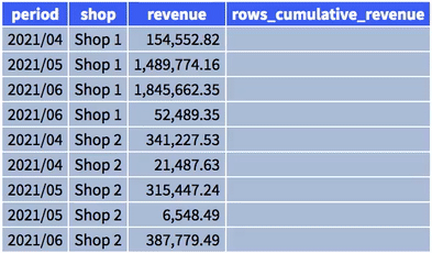
Now that we have some understanding of the sample data set, let's consider how using ROWS and RANGE can impact result sets for data we may want to report on. For example, suppose we want to calculate the cumulative revenue sum for every shop. Let's do this first with ROWS and then with RANGE and observe the differences in behavior.
ROWS
The ROWS units of a frame clause means a window frame will be defined as the number of rows preceding and/or following the current row.
- Query
- Result set (static)
- Result set (animated)
SELECT
  period,
  shop,
  revenue,
  SUM(revenue) OVER(
    PARTITION BY shop
    ORDER BY period ASC
    # highlight-next-line
    ROWS UNBOUNDED PRECEDING
  ) AS rows_cumulative_revenue
FROM revenue_consolidation;
Note: Highlighted lines below indicate cumulative revenue value differentials compared to corresponding entries when using
RANGE.
+---------+--------+------------+-------------------------+
| period  | shop   | revenue    | rows_cumulative_revenue |
+---------+--------+------------+-------------------------+
| 2021/04 | Shop 1 |  154552.82 |               154552.82 |
| 2021/05 | Shop 1 | 1489774.16 |              1644326.98 |
| 2021/06 | Shop 1 | 1845662.35 |              3489989.33 |
| 2021/06 | Shop 1 |   52489.35 |              3542478.68 |
| 2021/04 | Shop 2 |  341227.53 |               341227.53 |
| 2021/04 | Shop 2 |   21487.63 |               362715.16 |
| 2021/05 | Shop 2 |  315447.24 |               678162.40 |
| 2021/05 | Shop 2 |    6548.49 |               684710.89 |
| 2021/06 | Shop 2 |  387779.49 |              1072490.38 |
+---------+--------+------------+-------------------------+
Let's explore what manually computing the result set above would look like. The principle computation is as follows:
Hence, for the first row, the calculation is
which is exactly what we see in the result set above. For the second row, we have
1489774.16 + 154552.82 = 1644326.98
Similarly, for the third row we have
1845662.35 + 1644326.98 = 3489989.33
We continue doing this for all Shop 1 rows. Once we come to the Shop 2 rows, we restart the process, starting with the first row in the partition:
341227.53 + 0 = 341227.53
And so on until we reach the end of the table. The far-right tab above provides an animation of this computational process.
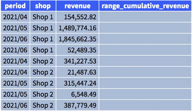
RANGE
The RANGE units of a frame clause means a window frame will be defined by the number of rows preceding and/or following the current row plus all other rows that have the same value.
- Query
- Result set (static)
- Result set (animated)
SELECT
  period,
  shop,
  revenue,
  SUM(revenue) OVER(
    PARTITION BY shop
    ORDER BY period ASC
    # highlight-next-line
    RANGE UNBOUNDED PRECEDING
  ) AS range_cumulative_revenue
FROM revenue_consolidation;
Note: Highlighted lines below indicate cumulative revenue value differentials compared to corresponding entries when using
ROWS.
+---------+--------+------------+--------------------------+
| period  | shop   | revenue    | range_cumulative_revenue |
+---------+--------+------------+--------------------------+
| 2021/04 | Shop 1 |  154552.82 |                154552.82 |
| 2021/05 | Shop 1 | 1489774.16 |               1644326.98 |
| 2021/06 | Shop 1 | 1845662.35 |               3542478.68 |
| 2021/06 | Shop 1 |   52489.35 |               3542478.68 |
| 2021/04 | Shop 2 |  341227.53 |                362715.16 |
| 2021/04 | Shop 2 |   21487.63 |                362715.16 |
| 2021/05 | Shop 2 |  315447.24 |                684710.89 |
| 2021/05 | Shop 2 |    6548.49 |                684710.89 |
| 2021/06 | Shop 2 |  387779.49 |               1072490.38 |
+---------+--------+------------+--------------------------+
Let's explore what manually computing the result set above would look like. It may help to first look at the animation of this computational process in the far-right tab above. Essentially, the RANGE clause makes use of the following:
- all previous rows (i.e.,
UNBOUNDED PRECEDING), - the current row (i.e.,
RANGE UNBOUNDED PRECEDINGis shorthand forRANGE BETWEEN UNBOUNDED PRECEDING AND CURRENT ROW), and - all other rows that contain the revenue for the current partition (i.e.,
Shop 1orStep 2) and currentperiod(e.g.,2021/06).
The manual calculation looks somewhat similar to that of the one with ROWS, but the twist occurs in the third bullet point above. Specifically, nothing special happens in this example for the first row:
154552.82 + 0 = 154552.82
Or even the second row:
1489774.16 + 154552.82 = 1644326.98
Everything so far is the same as it was with ROWS. But now is where we encounter the twist. The next two rows both contain revenue for the period of 2021/06 for Shop 1. Both rows will be treated together since they are part of the same partition (i.e., Shop 1) and they have the same value for the field by which rows are being ordered (i.e., period); that is, both rows will be treated together by summing their revenue values, which matches how it works in the real world in that there should only be one cumulative value at the end of each month.
The computational principle at work here is as follows:
Hence, we have
1845662.35 + 52489.35 + 1644326.98 = 3542478.68
for when we encounter the period of 2021/06 of the Shop 1 partition. This is the cumulative revenue for Shop 1 for the period 2021/06, and the same value appears in both rows; that is, the cumulative revenue is obtained and then the same value is replicated for all rows of the same shop and month. See the far-right tab above for an animation of the computational process.
Example 1 (problem-based with extended discussion)
- Problem
- Solution
- single_order
- Schema
- Extended Discussion
Calculate the running sum for all orders in the single_order table (sorted by date). The result set should include columns id, placed, total_price, and running_sum.
One approach might be to try to use ROWS UNBOUNDED PRECEDING as the window function frame clause:
SELECT
  id,
  placed,
  total_price,
  # highlight-next-line
  SUM(total_price) OVER(ORDER BY placed ROWS UNBOUNDED PRECEDING) AS running_sum
FROM single_order;
+------+------------+-------------+-------------+
| id   | placed     | total_price | running_sum |
+------+------------+-------------+-------------+
|    4 | 2016-06-13 |     2659.63 |     2659.63 |
|    5 | 2016-06-13 |      602.03 |     3261.66 |
|    6 | 2016-06-13 |     3599.83 |     6861.49 |
|    7 | 2016-06-29 |     4402.04 |    11263.53 |
|    1 | 2016-07-10 |     3876.76 |    15140.29 |
|    2 | 2016-07-10 |     3949.21 |    19089.50 |
|    3 | 2016-07-18 |     2199.46 |    21288.96 |
|   10 | 2016-08-01 |     4973.43 |    26262.39 |
|   11 | 2016-08-05 |     3252.83 |    29515.22 |
|   12 | 2016-08-05 |     3796.42 |    33311.64 |
|    8 | 2016-08-21 |     4553.89 |    37865.53 |
|    9 | 2016-08-30 |     3575.55 |    41441.08 |
+------+------------+-------------+-------------+
This may work fine in some sense, but our boss may very well say, "Hey, I don't really need to see how the running sum changed during single days (highlighted lines above). Just show the values at the end of the day. If there are multiple orders on a single day, then add or lump them together."
Using RANGE UNBOUNDED PRECEDING fixes this problem:
SELECT
  id,
  placed,
  total_price,
  # highlight-next-line
  SUM(total_price) OVER(ORDER BY placed RANGE UNBOUNDED PRECEDING) AS running_sum
FROM single_order;
+------+------------+-------------+-------------+
| id   | placed     | total_price | running_sum |
+------+------------+-------------+-------------+
|    4 | 2016-06-13 |     2659.63 |     6861.49 |
|    5 | 2016-06-13 |      602.03 |     6861.49 |
|    6 | 2016-06-13 |     3599.83 |     6861.49 |
|    7 | 2016-06-29 |     4402.04 |    11263.53 |
|    1 | 2016-07-10 |     3876.76 |    19089.50 |
|    2 | 2016-07-10 |     3949.21 |    19089.50 |
|    3 | 2016-07-18 |     2199.46 |    21288.96 |
|   10 | 2016-08-01 |     4973.43 |    26262.39 |
|   11 | 2016-08-05 |     3252.83 |    33311.64 |
|   12 | 2016-08-05 |     3796.42 |    33311.64 |
|    8 | 2016-08-21 |     4553.89 |    37865.53 |
|    9 | 2016-08-30 |     3575.55 |    41441.08 |
+------+------------+-------------+-------------+
The default window frame clause when ORDER BY is used in the window frame specification is RANGE UNBOUNDED PRECEDING; hence, the line
SUM(total_price) OVER(ORDER BY placed RANGE UNBOUNDED PRECEDING) AS running_sum
could more concisely be expressed as follows:
SUM(total_price) OVER(ORDER BY placed) AS running_sum
If ORDER BY were not used, then
RANGE BETWEEN UNBOUNDED PRECEDING AND UNBOUNDED FOLLOWING
would be the default frame clause (i.e., the entire partition would be the frame).
This example shows how the choice of frame units ROWS and RANGE can strongly impact the ultimate result set returned: RANGE will take into account all rows that have the same value in the column(s) which we order by. See the "Extended Discussion" tab for an example where RANGE is used when more than one column is being used to order rows within a partition.
+------+------------+-------------+
| id   | placed     | total_price |
+------+------------+-------------+
|    1 | 2016-07-10 |     3876.76 |
|    2 | 2016-07-10 |     3949.21 |
|    3 | 2016-07-18 |     2199.46 |
|    4 | 2016-06-13 |     2659.63 |
|    5 | 2016-06-13 |      602.03 |
|    6 | 2016-06-13 |     3599.83 |
|    7 | 2016-06-29 |     4402.04 |
|    8 | 2016-08-21 |     4553.89 |
|    9 | 2016-08-30 |     3575.55 |
|   10 | 2016-08-01 |     4973.43 |
|   11 | 2016-08-05 |     3252.83 |
|   12 | 2016-08-05 |     3796.42 |
+------+------------+-------------+
DROP TABLE IF EXISTS single_order;

CREATE TABLE IF NOT EXISTS
  single_order (id INT, placed DATE, total_price DECIMAL(10,2));

INSERT INTO
  single_order (id, placed, total_price)
VALUES
  (1, '2016-07-10', 3876.76),
  (2, '2016-07-10', 3949.21),
  (3, '2016-07-18', 2199.46),
  (4, '2016-06-13', 2659.63),
  (5, '2016-06-13', 602.03),
  (6, '2016-06-13', 3599.83),
  (7, '2016-06-29', 4402.04),
  (8, '2016-08-21', 4553.89),
  (9, '2016-08-30', 3575.55),
  (10, '2016-08-01', 4973.43),
  (11, '2016-08-05', 3252.83),
  (12, '2016-08-05', 3796.42);
So far we have only dealt with scenarios where a single field is being used to ORDER BY within a window function, but it will often be the case that we use more than one field. How can we expect RANGE to behave in such instances? The answer may depend on your RDBMS (always read the docs!), but the behavior described in the Solution tab for this example can be expected to extend to multi-column orderings:
The difference between
ROWSandRANGEis thatRANGEwill take into account all rows that have the same value in the column(s) which we order by.
The column(s) part is important. We are interested in more than a single column now. To illustrate how RANGE will take into account all rows that have the same value in the columns which we order by, we will add a other_id field to the single_order table, query the results by order by not only placed but also by other_id, and we will observe the differences in output (noteworthy lines have been highlighted):
DROP TABLE IF EXISTS single_order;

CREATE TABLE IF NOT EXISTS
  single_order (id INT, other_id INT, placed DATE, total_price DECIMAL(10,2));

INSERT INTO
  single_order (id, other_id, placed, total_price)
VALUES
  # highlight-start
  (1, 1, '2016-07-10', 3876.76),
  (2, 2, '2016-07-10', 3949.21),
  # highlight-end
  (3, 3, '2016-07-18', 2199.46),
  # highlight-start
  (4, 4, '2016-06-13', 2659.63),
  (5, 4, '2016-06-13', 602.03),
  (6, 4, '2016-06-13', 3599.83),
  # highlight-end
  (7, 5, '2016-06-29', 4402.04),
  (8, 6, '2016-08-21', 4553.89),
  (9, 7, '2016-08-30', 3575.55),
  (10, 8, '2016-08-01', 4973.43),
  (11, 9, '2016-08-05', 3252.83),
  (12, 9, '2016-08-05', 3796.42);
SELECT
  id,
  other_id,
  placed,
  total_price,
  # highlight-next-line
  SUM(total_price) OVER(ORDER BY placed, other_id RANGE UNBOUNDED PRECEDING) AS running_sum
FROM single_order;
+------+----------+------------+-------------+-------------+
| id   | other_id | placed     | total_price | running_sum |
+------+----------+------------+-------------+-------------+
|    4 |        4 | 2016-06-13 |     2659.63 |     6861.49 |
|    5 |        4 | 2016-06-13 |      602.03 |     6861.49 |
|    6 |        4 | 2016-06-13 |     3599.83 |     6861.49 |
|    7 |        5 | 2016-06-29 |     4402.04 |    11263.53 |
|    1 |        1 | 2016-07-10 |     3876.76 |    15140.29 |
|    2 |        2 | 2016-07-10 |     3949.21 |    19089.50 |
|    3 |        3 | 2016-07-18 |     2199.46 |    21288.96 |
|   10 |        8 | 2016-08-01 |     4973.43 |    26262.39 |
|   11 |        9 | 2016-08-05 |     3252.83 |    33311.64 |
|   12 |        9 | 2016-08-05 |     3796.42 |    33311.64 |
|    8 |        6 | 2016-08-21 |     4553.89 |    37865.53 |
|    9 |        7 | 2016-08-30 |     3575.55 |    41441.08 |
+------+----------+------------+-------------+-------------+
The highlighted lines in the result set above show how RANGE groups the records with equivalent placed and other_id values (the columns which we are ordering by in the window specification). Even though the second block of highlighted lines have the same placed date (i.e., 2016-07-10), these records do not have the same other_id value and are thus not grouped by RANGE.
For completeness, it is worth noting that using ROWS always leads to the expected behavior:
+------+----------+------------+-------------+-------------+
| id   | other_id | placed     | total_price | running_sum |
+------+----------+------------+-------------+-------------+
|    4 |        4 | 2016-06-13 |     2659.63 |     2659.63 |
|    5 |        4 | 2016-06-13 |      602.03 |     3261.66 |
|    6 |        4 | 2016-06-13 |     3599.83 |     6861.49 |
|    7 |        5 | 2016-06-29 |     4402.04 |    11263.53 |
|    1 |        1 | 2016-07-10 |     3876.76 |    15140.29 |
|    2 |        2 | 2016-07-10 |     3949.21 |    19089.50 |
|    3 |        3 | 2016-07-18 |     2199.46 |    21288.96 |
|   10 |        8 | 2016-08-01 |     4973.43 |    26262.39 |
|   11 |        9 | 2016-08-05 |     3252.83 |    29515.22 |
|   12 |        9 | 2016-08-05 |     3796.42 |    33311.64 |
|    8 |        6 | 2016-08-21 |     4553.89 |    37865.53 |
|    9 |        7 | 2016-08-30 |     3575.55 |    41441.08 |
+------+----------+------------+-------------+-------------+
Example 2 (ROWS, number of orders up to current order)
- Problem
- Solution
- single_order
- Schema
For each order from the single_order table, show the order's id, the placed date, and count which should show the count of the number of orders up to the current order when sorted by the placed date.
Use the COUNT() window function and ROWS in your solution.
SELECT
	id,
  placed,
  COUNT(id) OVER(ORDER BY placed ROWS UNBOUNDED PRECEDING) AS count
FROM
	single_order
ORDER BY placed;
+------+------------+-------+
| id   | placed     | count |
+------+------------+-------+
|    4 | 2016-06-13 |     1 |
|    5 | 2016-06-13 |     2 |
|    6 | 2016-06-13 |     3 |
|    7 | 2016-06-29 |     4 |
|    1 | 2016-07-10 |     5 |
|    2 | 2016-07-10 |     6 |
|    3 | 2016-07-18 |     7 |
|   10 | 2016-08-01 |     8 |
|   11 | 2016-08-05 |     9 |
|   12 | 2016-08-05 |    10 |
|    8 | 2016-08-21 |    11 |
|    9 | 2016-08-30 |    12 |
+------+------------+-------+
It might be tempting to try the solution query without modifying the frame clause:
SELECT
	id,
  placed,
  # highlight-next-line
  COUNT(id) OVER(ORDER BY placed) AS count
FROM
	single_order
ORDER BY placed;
But the result set returned is all wrong:
+------+------------+-------+
| id   | placed     | count |
+------+------------+-------+
|    4 | 2016-06-13 |     3 |
|    5 | 2016-06-13 |     3 |
|    6 | 2016-06-13 |     3 |
|    7 | 2016-06-29 |     4 |
|    1 | 2016-07-10 |     6 |
|    2 | 2016-07-10 |     6 |
|    3 | 2016-07-18 |     7 |
|   10 | 2016-08-01 |     8 |
|   11 | 2016-08-05 |    10 |
|   12 | 2016-08-05 |    10 |
|    8 | 2016-08-21 |    11 |
|    9 | 2016-08-30 |    12 |
+------+------------+-------+
This is because the default frame specification used when ORDER BY is included is RANGE UNBOUNDED PRECEDING which implicitly groups the first three row entries because their placed value is equivalent (i.e., 2016-06-13).
A "normal" solution might be to use the ROW_NUMBER() window function:
SELECT
	id,
  placed,
  ROW_NUMBER() OVER(ORDER BY placed) AS count
FROM
	single_order
ORDER BY placed;
This produces the desired result set without having to modify the default frame clause, but using COUNT() as a window function seems more natural in this case (along with being a requirement). It simply means we have to exercise caution when considering what the default frame specification definition may be if we do not modify it ourselves.
+------+------------+-------------+
| id   | placed     | total_price |
+------+------------+-------------+
|    1 | 2016-07-10 |     3876.76 |
|    2 | 2016-07-10 |     3949.21 |
|    3 | 2016-07-18 |     2199.46 |
|    4 | 2016-06-13 |     2659.63 |
|    5 | 2016-06-13 |      602.03 |
|    6 | 2016-06-13 |     3599.83 |
|    7 | 2016-06-29 |     4402.04 |
|    8 | 2016-08-21 |     4553.89 |
|    9 | 2016-08-30 |     3575.55 |
|   10 | 2016-08-01 |     4973.43 |
|   11 | 2016-08-05 |     3252.83 |
|   12 | 2016-08-05 |     3796.42 |
+------+------------+-------------+
DROP TABLE IF EXISTS single_order;

CREATE TABLE IF NOT EXISTS
  single_order (id INT, placed DATE, total_price DECIMAL(10,2));

INSERT INTO
  single_order (id, placed, total_price)
VALUES
  (1, '2016-07-10', 3876.76),
  (2, '2016-07-10', 3949.21),
  (3, '2016-07-18', 2199.46),
  (4, '2016-06-13', 2659.63),
  (5, '2016-06-13', 602.03),
  (6, '2016-06-13', 3599.83),
  (7, '2016-06-29', 4402.04),
  (8, '2016-08-21', 4553.89),
  (9, '2016-08-30', 3575.55),
  (10, '2016-08-01', 4973.43),
  (11, '2016-08-05', 3252.83),
  (12, '2016-08-05', 3796.42);
Example 3 (ROWS, quantity of remaining items)
- Problem
- Solution
- order_position
- Schema
Warehouse workers always need to pick the products for orders by hand and one by one. For positions with order_id = 5 in the order_position table, calculate the remaining sum of all the products to pick. Specifically, for each position from orders with order_id = 5, show the position's id, product_id, quantity, and, most importantly, sum, the quantity of the remaining items (including the current row) when sorted by position id in ascending order.
Use the SUM() window function and ROWS in your solution.
SELECT
  id,
  product_id,
  quantity,
  SUM(quantity) OVER(ORDER BY id ROWS BETWEEN CURRENT ROW AND UNBOUNDED FOLLOWING) AS sum
FROM order_position
WHERE order_id = 5;
+------+------------+----------+------+
| id   | product_id | quantity | sum  |
+------+------------+----------+------+
|    5 |          1 |       16 |   77 |
|   20 |          6 |       21 |   61 |
|   26 |          5 |        4 |   40 |
|   33 |          4 |        5 |   36 |
|   35 |          6 |       29 |   31 |
|   44 |          5 |        2 |    2 |
+------+------------+----------+------+
+------+------------+----------+----------+
| id   | product_id | order_id | quantity |
+------+------------+----------+----------+
|    1 |          1 |        9 |        7 |
|    2 |          1 |        6 |       15 |
|    3 |          7 |        2 |        1 |
|    4 |          1 |        4 |       24 |
|    5 |          1 |        5 |       16 |
|    6 |          3 |        8 |        7 |
|    7 |          5 |       12 |        5 |
|    8 |          2 |       12 |        1 |
|    9 |          5 |       10 |       20 |
|   10 |          2 |        8 |       14 |
|   11 |          4 |        6 |       28 |
|   12 |          6 |        3 |       15 |
|   13 |          6 |        6 |       16 |
|   14 |          4 |        1 |        8 |
|   15 |          2 |        8 |       13 |
|   16 |          5 |        4 |       27 |
|   17 |          2 |        8 |       30 |
|   18 |          7 |        6 |       29 |
|   19 |          1 |       10 |        6 |
|   20 |          6 |        5 |       21 |
|   21 |          1 |       11 |        9 |
|   22 |          6 |        7 |        4 |
|   23 |          5 |        8 |       27 |
|   24 |          7 |        1 |       25 |
|   25 |          4 |        3 |       16 |
|   26 |          5 |        5 |        4 |
|   27 |          4 |        6 |        1 |
|   28 |          2 |        6 |        5 |
|   29 |          5 |        4 |       29 |
|   30 |          4 |       11 |       21 |
|   31 |          4 |       10 |       18 |
|   32 |          6 |        1 |        5 |
|   33 |          4 |        5 |        5 |
|   34 |          3 |       12 |       19 |
|   35 |          6 |        5 |       29 |
|   36 |          5 |        9 |       21 |
|   37 |          6 |        7 |       25 |
|   38 |          4 |        4 |        3 |
|   39 |          6 |        9 |       21 |
|   40 |          3 |        4 |       15 |
|   41 |          6 |       12 |       17 |
|   42 |          2 |        3 |       18 |
|   43 |          2 |        7 |       30 |
|   44 |          5 |        5 |        2 |
|   45 |          6 |        3 |       26 |
|   46 |          3 |        3 |       13 |
|   47 |          2 |        8 |       29 |
|   48 |          7 |       11 |       26 |
|   49 |          3 |        8 |       12 |
|   50 |          3 |        6 |        4 |
+------+------------+----------+----------+
DROP TABLE IF EXISTS order_position;

CREATE TABLE IF NOT EXISTS
  order_position (id INT, product_id INT, order_id INT, quantity INT);

INSERT INTO
  order_position (id, product_id, order_id, quantity)
VALUES
  (1,1,9,7),
  (2,1,6,15),
  (3,7,2,1),
  (4,1,4,24),
  (5,1,5,16),
  (6,3,8,7),
  (7,5,12,5),
  (8,2,12,1),
  (9,5,10,20),
  (10,2,8,14),
  (11,4,6,28),
  (12,6,3,15),
  (13,6,6,16),
  (14,4,1,8),
  (15,2,8,13),
  (16,5,4,27),
  (17,2,8,30),
  (18,7,6,29),
  (19,1,10,6),
  (20,6,5,21),
  (21,1,11,9),
  (22,6,7,4),
  (23,5,8,27),
  (24,7,1,25),
  (25,4,3,16),
  (26,5,5,4),
  (27,4,6,1),
  (28,2,6,5),
  (29,5,4,29),
  (30,4,11,21),
  (31,4,10,18),
  (32,6,1,5),
  (33,4,5,5),
  (34,3,12,19),
  (35,6,5,29),
  (36,5,9,21),
  (37,6,7,25),
  (38,4,4,3),
  (39,6,9,21),
  (40,3,4,15),
  (41,6,12,17),
  (42,2,3,18),
  (43,2,7,30),
  (44,5,5,2),
  (45,6,3,26),
  (46,3,3,13),
  (47,2,8,29),
  (48,7,11,26),
  (49,3,8,12),
  (50,3,6,4);
Example 4 (ROWS, count of products introduced up to a point)
- Problem
- Solution
- product
- Schema
For each product from the product table, show the product's id, name, introduced date and count, the count of products introduced up to that point (ordered by introduced date in ascending order).
Use the COUNT() window function and ROWS in your solution.
SELECT
  id,
  name,
  introduced,
  COUNT(id) OVER(ORDER BY introduced ROWS UNBOUNDED PRECEDING) AS count
FROM
  product;
+------+----------------+------------+-------+
| id   | name           | introduced | count |
+------+----------------+------------+-------+
|    3 | Ice cream      | 2016-01-05 |     1 |
|    7 | Freezer        | 2016-01-16 |     2 |
|    1 | Frozen Yoghurt | 2016-01-26 |     3 |
|    5 | Snowboard      | 2016-02-01 |     4 |
|    6 | Sledge         | 2016-02-20 |     5 |
|    4 | Skis           | 2016-04-09 |     6 |
|    2 | Ice cubes      | 2016-04-10 |     7 |
+------+----------------+------------+-------+
+------+----------------+------------+
| id   | name           | introduced |
+------+----------------+------------+
|    1 | Frozen Yoghurt | 2016-01-26 |
|    2 | Ice cubes      | 2016-04-10 |
|    3 | Ice cream      | 2016-01-05 |
|    4 | Skis           | 2016-04-09 |
|    5 | Snowboard      | 2016-02-01 |
|    6 | Sledge         | 2016-02-20 |
|    7 | Freezer        | 2016-01-16 |
+------+----------------+------------+
DROP TABLE IF EXISTS product;

CREATE TABLE IF NOT EXISTS
  product (id INT, name VARCHAR(20), introduced DATE);

INSERT INTO
  product (id, name, introduced)
VALUES
  (1, 'Frozen Yoghurt', '2016-01-26'),
  (2, 'Ice cubes', '2016-04-10'),
  (3, 'Ice cream', '2016-01-05'),
  (4, 'Skis', '2016-04-09'),
  (5, 'Snowboard', '2016-02-01'),
  (6, 'Sledge', '2016-02-20'),
  (7, 'Freezer', '2016-01-16');
Example 5 (ROWS, moving average)
- Problem
- Solution
- single_order
- Schema
For each order from the single_order table, show the order's placed date, total_price, average price avg calculated by taking 2 previous orders, the current order, and the 2 following orders (in terms of the placed date), and the ratio of the total_price to avg calculated above.
Use the AVG() window function and ROWS in your solution.
SELECT
	placed,
  total_price,
  AVG(total_price) OVER(ORDER BY placed ROWS BETWEEN 2 PRECEDING AND 2 FOLLOWING) AS avg,
  total_price / AVG(total_price) OVER(ORDER BY placed ROWS BETWEEN 2 PRECEDING AND 2 FOLLOWING) AS ratio
FROM
	single_order;
+------------+-------------+-------------+----------+
| placed     | total_price | avg         | ratio    |
+------------+-------------+-------------+----------+
| 2016-06-13 |     2659.63 | 2287.163333 | 1.162851 |
| 2016-06-13 |      602.03 | 2815.882500 | 0.213798 |
| 2016-06-13 |     3599.83 | 3028.058000 | 1.188825 |
| 2016-06-29 |     4402.04 | 3285.974000 | 1.339645 |
| 2016-07-10 |     3876.76 | 3605.460000 | 1.075247 |
| 2016-07-10 |     3949.21 | 3880.180000 | 1.017790 |
| 2016-07-18 |     2199.46 | 3650.338000 | 0.602536 |
| 2016-08-01 |     4973.43 | 3634.270000 | 1.368481 |
| 2016-08-05 |     3252.83 | 3755.206000 | 0.866219 |
| 2016-08-05 |     3796.42 | 4030.424000 | 0.941941 |
| 2016-08-21 |     4553.89 | 3794.672500 | 1.200075 |
| 2016-08-30 |     3575.55 | 3975.286667 | 0.899445 |
+------------+-------------+-------------+----------+
+------+------------+-------------+
| id   | placed     | total_price |
+------+------------+-------------+
|    1 | 2016-07-10 |     3876.76 |
|    2 | 2016-07-10 |     3949.21 |
|    3 | 2016-07-18 |     2199.46 |
|    4 | 2016-06-13 |     2659.63 |
|    5 | 2016-06-13 |      602.03 |
|    6 | 2016-06-13 |     3599.83 |
|    7 | 2016-06-29 |     4402.04 |
|    8 | 2016-08-21 |     4553.89 |
|    9 | 2016-08-30 |     3575.55 |
|   10 | 2016-08-01 |     4973.43 |
|   11 | 2016-08-05 |     3252.83 |
|   12 | 2016-08-05 |     3796.42 |
+------+------------+-------------+
DROP TABLE IF EXISTS single_order;

CREATE TABLE IF NOT EXISTS
  single_order (id INT, placed DATE, total_price DECIMAL(10,2));

INSERT INTO
  single_order (id, placed, total_price)
VALUES
  (1, '2016-07-10', 3876.76),
  (2, '2016-07-10', 3949.21),
  (3, '2016-07-18', 2199.46),
  (4, '2016-06-13', 2659.63),
  (5, '2016-06-13', 602.03),
  (6, '2016-06-13', 3599.83),
  (7, '2016-06-29', 4402.04),
  (8, '2016-08-21', 4553.89),
  (9, '2016-08-30', 3575.55),
  (10, '2016-08-01', 4973.43),
  (11, '2016-08-05', 3252.83),
  (12, '2016-08-05', 3796.42);
Example 6 (RANGE, daily average)
- Problem
- Solution
- single_order
- Schema
Calculate the average total_price for orders in the single_order table (sorted by date and reported for single days; that is, the average reported should not be different for the same day). The result set should include columns id, placed, total_price, and avg.
Use RANGE in your solution.
SELECT
  id,
  placed,
  total_price,
  AVG(total_price) OVER(ORDER BY placed RANGE CURRENT ROW) AS avg
FROM single_order;
+------+------------+-------------+-------------+
| id   | placed     | total_price | avg         |
+------+------------+-------------+-------------+
|    4 | 2016-06-13 |     2659.63 | 2287.163333 |
|    5 | 2016-06-13 |      602.03 | 2287.163333 |
|    6 | 2016-06-13 |     3599.83 | 2287.163333 |
|    7 | 2016-06-29 |     4402.04 | 4402.040000 |
|    1 | 2016-07-10 |     3876.76 | 3912.985000 |
|    2 | 2016-07-10 |     3949.21 | 3912.985000 |
|    3 | 2016-07-18 |     2199.46 | 2199.460000 |
|   10 | 2016-08-01 |     4973.43 | 4973.430000 |
|   11 | 2016-08-05 |     3252.83 | 3524.625000 |
|   12 | 2016-08-05 |     3796.42 | 3524.625000 |
|    8 | 2016-08-21 |     4553.89 | 4553.890000 |
|    9 | 2016-08-30 |     3575.55 | 3575.550000 |
+------+------------+-------------+-------------+
Note the difference between the above query and result set and what would have happened if we simply used AVG(total_price) OVER(ORDER BY placed), which uses a window frame definition of RANGE UNBOUNDED PRECEDING by default:
SELECT
  id,
  placed,
  total_price,
  AVG(total_price) OVER(ORDER BY placed) AS avg
FROM single_order;
+------+------------+-------------+-------------+
| id   | placed     | total_price | avg         |
+------+------------+-------------+-------------+
|    4 | 2016-06-13 |     2659.63 | 2287.163333 |
|    5 | 2016-06-13 |      602.03 | 2287.163333 |
|    6 | 2016-06-13 |     3599.83 | 2287.163333 |
|    7 | 2016-06-29 |     4402.04 | 2815.882500 |
|    1 | 2016-07-10 |     3876.76 | 3181.583333 |
|    2 | 2016-07-10 |     3949.21 | 3181.583333 |
|    3 | 2016-07-18 |     2199.46 | 3041.280000 |
|   10 | 2016-08-01 |     4973.43 | 3282.798750 |
|   11 | 2016-08-05 |     3252.83 | 3331.164000 |
|   12 | 2016-08-05 |     3796.42 | 3331.164000 |
|    8 | 2016-08-21 |     4553.89 | 3442.320909 |
|    9 | 2016-08-30 |     3575.55 | 3453.423333 |
+------+------------+-------------+-------------+
Recall that the goal was to find the average total_price for single days for each row. The default frame clause of RANGE UNBOUNDED PRECEDING, which is shorthand for
RANGE BETWEEN UNBOUNDED PRECEDING AND CURRENT ROW
does not lead to the calculations we want. Specifically, for the lines highlighted in the result sets above, we can tell the line
| 7 | 2016-06-29 | 4402.04 | 2815.882500 |
from the second result set is incorrect because this record is the lone entry for a placed date of 2016-06-29. This line should have an avg value of 4402.04, but the value of 2815.882500 comes from the following calculation:
The correct frame clause of RANGE CURRENT ROW is shorthand for
RANGE BETWEEN CURRENT ROW AND CURRENT ROW
which, based on the grouping behavior of RANGE, results in computing the proper average for each placed date (RANGE groups records by equivalent placed values since that is the field being ordered by in the window specification).
+------+------------+-------------+
| id   | placed     | total_price |
+------+------------+-------------+
|    1 | 2016-07-10 |     3876.76 |
|    2 | 2016-07-10 |     3949.21 |
|    3 | 2016-07-18 |     2199.46 |
|    4 | 2016-06-13 |     2659.63 |
|    5 | 2016-06-13 |      602.03 |
|    6 | 2016-06-13 |     3599.83 |
|    7 | 2016-06-29 |     4402.04 |
|    8 | 2016-08-21 |     4553.89 |
|    9 | 2016-08-30 |     3575.55 |
|   10 | 2016-08-01 |     4973.43 |
|   11 | 2016-08-05 |     3252.83 |
|   12 | 2016-08-05 |     3796.42 |
+------+------------+-------------+
DROP TABLE IF EXISTS single_order;

CREATE TABLE IF NOT EXISTS
  single_order (id INT, placed DATE, total_price DECIMAL(10,2));

INSERT INTO
  single_order (id, placed, total_price)
VALUES
  (1, '2016-07-10', 3876.76),
  (2, '2016-07-10', 3949.21),
  (3, '2016-07-18', 2199.46),
  (4, '2016-06-13', 2659.63),
  (5, '2016-06-13', 602.03),
  (6, '2016-06-13', 3599.83),
  (7, '2016-06-29', 4402.04),
  (8, '2016-08-21', 4553.89),
  (9, '2016-08-30', 3575.55),
  (10, '2016-08-01', 4973.43),
  (11, '2016-08-05', 3252.83),
  (12, '2016-08-05', 3796.42);
Example 7 (RANGE, number of stock changes for a day)
- Problem
- Solution
- Data set
- Schema
For each stock_change from the stock_change table with product_id = 7, show the stock change's id, quantity, changed date and another column count which will count the number of stock changes with product_id = 7 on that particular date.
Use RANGE in your solution.
SELECT
  id,
  quantity,
  changed,
  COUNT(id) OVER(ORDER BY changed RANGE CURRENT ROW) AS count
FROM
  stock_change
WHERE
  product_id = 7;
+------+----------+------------+-------+
| id   | quantity | changed    | count |
+------+----------+------------+-------+
|   14 |       19 | 2016-07-14 |     1 |
|   16 |      -13 | 2016-08-28 |     1 |
|   15 |      -72 | 2016-09-13 |     1 |
+------+----------+------------+-------+
+------+------------+----------+------------+
| id   | product_id | quantity | changed    |
+------+------------+----------+------------+
|    1 |          5 |      -90 | 2016-09-11 |
|    2 |          2 |      -91 | 2016-08-16 |
|    3 |          5 |      -15 | 2016-06-08 |
|    4 |          2 |       51 | 2016-06-10 |
|    5 |          1 |      -58 | 2016-08-09 |
|    6 |          1 |      -84 | 2016-09-28 |
|    7 |          4 |       56 | 2016-06-09 |
|    8 |          5 |       73 | 2016-09-22 |
|    9 |          1 |      -43 | 2016-06-07 |
|   10 |          2 |      -79 | 2016-07-27 |
|   11 |          4 |       93 | 2016-09-22 |
|   12 |          4 |       74 | 2016-06-13 |
|   13 |          2 |      -37 | 2016-08-02 |
|   14 |          7 |       19 | 2016-07-14 |
|   15 |          7 |      -72 | 2016-09-13 |
|   16 |          7 |      -13 | 2016-08-28 |
|   17 |          3 |       23 | 2016-07-24 |
|   18 |          1 |       24 | 2016-08-17 |
|   19 |          3 |       77 | 2016-08-11 |
|   20 |          1 |       24 | 2016-08-28 |
+------+------------+----------+------------+
DROP TABLE IF EXISTS stock_change;

CREATE TABLE IF NOT EXISTS
  stock_change (id INT, product_id INT, quantity INT, changed DATE);

INSERT INTO
  stock_change (id, product_id, quantity, changed)
VALUES
  (1, 5, -90, '2016-09-11'),
  (2, 2, -91, '2016-08-16'),
  (3, 5, -15, '2016-06-08'),
  (4, 2, 51, '2016-06-10'),
  (5, 1, -58, '2016-08-09'),
  (6, 1, -84, '2016-09-28'),
  (7, 4, 56, '2016-06-09'),
  (8, 5, 73, '2016-09-22'),
  (9, 1, -43, '2016-06-07'),
  (10, 2, -79, '2016-07-27'),
  (11, 4, 93, '2016-09-22'),
  (12, 4, 74, '2016-06-13'),
  (13, 2, -37, '2016-08-02'),
  (14, 7, 19, '2016-07-14'),
  (15, 7, -72, '2016-09-13'),
  (16, 7, -13, '2016-08-28'),
  (17, 3, 23, '2016-07-24'),
  (18, 1, 24, '2016-08-17'),
  (19, 3, 77, '2016-08-11'),
  (20, 1, 24, '2016-08-28');
Example 8 (RANGE, total quantity change for a product by date)
- Problem
- Solution
- Data set
- Schema
For each stock_change from the stock_change table, show the stock change's id, product_id, quantity, changed date, and sum, the total quantity change of stock changes for that product.
Use RANGE in your solution.
SELECT
  id,
  product_id,
  quantity,
  changed,
  SUM(quantity) OVER(ORDER BY product_id RANGE CURRENT ROW) AS sum
FROM
  stock_change;
+------+------------+----------+------------+------+
| id   | product_id | quantity | changed    | sum  |
+------+------------+----------+------------+------+
|    5 |          1 |      -58 | 2016-08-09 | -137 |
|    6 |          1 |      -84 | 2016-09-28 | -137 |
|    9 |          1 |      -43 | 2016-06-07 | -137 |
|   18 |          1 |       24 | 2016-08-17 | -137 |
|   20 |          1 |       24 | 2016-08-28 | -137 |
|    2 |          2 |      -91 | 2016-08-16 | -156 |
|    4 |          2 |       51 | 2016-06-10 | -156 |
|   10 |          2 |      -79 | 2016-07-27 | -156 |
|   13 |          2 |      -37 | 2016-08-02 | -156 |
|   17 |          3 |       23 | 2016-07-24 |  100 |
|   19 |          3 |       77 | 2016-08-11 |  100 |
|    7 |          4 |       56 | 2016-06-09 |  223 |
|   11 |          4 |       93 | 2016-09-22 |  223 |
|   12 |          4 |       74 | 2016-06-13 |  223 |
|    1 |          5 |      -90 | 2016-09-11 |  -32 |
|    3 |          5 |      -15 | 2016-06-08 |  -32 |
|    8 |          5 |       73 | 2016-09-22 |  -32 |
|   14 |          7 |       19 | 2016-07-14 |  -66 |
|   15 |          7 |      -72 | 2016-09-13 |  -66 |
|   16 |          7 |      -13 | 2016-08-28 |  -66 |
+------+------------+----------+------------+------+
+------+------------+----------+------------+
| id   | product_id | quantity | changed    |
+------+------------+----------+------------+
|    1 |          5 |      -90 | 2016-09-11 |
|    2 |          2 |      -91 | 2016-08-16 |
|    3 |          5 |      -15 | 2016-06-08 |
|    4 |          2 |       51 | 2016-06-10 |
|    5 |          1 |      -58 | 2016-08-09 |
|    6 |          1 |      -84 | 2016-09-28 |
|    7 |          4 |       56 | 2016-06-09 |
|    8 |          5 |       73 | 2016-09-22 |
|    9 |          1 |      -43 | 2016-06-07 |
|   10 |          2 |      -79 | 2016-07-27 |
|   11 |          4 |       93 | 2016-09-22 |
|   12 |          4 |       74 | 2016-06-13 |
|   13 |          2 |      -37 | 2016-08-02 |
|   14 |          7 |       19 | 2016-07-14 |
|   15 |          7 |      -72 | 2016-09-13 |
|   16 |          7 |      -13 | 2016-08-28 |
|   17 |          3 |       23 | 2016-07-24 |
|   18 |          1 |       24 | 2016-08-17 |
|   19 |          3 |       77 | 2016-08-11 |
|   20 |          1 |       24 | 2016-08-28 |
+------+------------+----------+------------+
DROP TABLE IF EXISTS stock_change;

CREATE TABLE IF NOT EXISTS
  stock_change (id INT, product_id INT, quantity INT, changed DATE);

INSERT INTO
  stock_change (id, product_id, quantity, changed)
VALUES
  (1, 5, -90, '2016-09-11'),
  (2, 2, -91, '2016-08-16'),
  (3, 5, -15, '2016-06-08'),
  (4, 2, 51, '2016-06-10'),
  (5, 1, -58, '2016-08-09'),
  (6, 1, -84, '2016-09-28'),
  (7, 4, 56, '2016-06-09'),
  (8, 5, 73, '2016-09-22'),
  (9, 1, -43, '2016-06-07'),
  (10, 2, -79, '2016-07-27'),
  (11, 4, 93, '2016-09-22'),
  (12, 4, 74, '2016-06-13'),
  (13, 2, -37, '2016-08-02'),
  (14, 7, 19, '2016-07-14'),
  (15, 7, -72, '2016-09-13'),
  (16, 7, -13, '2016-08-28'),
  (17, 3, 23, '2016-07-24'),
  (18, 1, 24, '2016-08-17'),
  (19, 3, 77, '2016-08-11'),
  (20, 1, 24, '2016-08-28');
Example 9 (RANGE, number of stock changes for all products up through a date)
- Problem
- Solution
- Data set
- Schema
For each stock_change from the stock_change table, show the stock change's id, changed date, and count, the number of stock changes for all products that took place on the same day or any time earlier.
Use RANGE in your solution.
SELECT
  id,
  changed,
  COUNT(id) OVER(ORDER BY changed RANGE UNBOUNDED PRECEDING) AS count
FROM
  stock_change;
+------+------------+-------+
| id   | changed    | count |
+------+------------+-------+
|    9 | 2016-06-07 |     1 |
|    3 | 2016-06-08 |     2 |
|    7 | 2016-06-09 |     3 |
|    4 | 2016-06-10 |     4 |
|   12 | 2016-06-13 |     5 |
|   14 | 2016-07-14 |     6 |
|   17 | 2016-07-24 |     7 |
|   10 | 2016-07-27 |     8 |
|   13 | 2016-08-02 |     9 |
|    5 | 2016-08-09 |    10 |
|   19 | 2016-08-11 |    11 |
|    2 | 2016-08-16 |    12 |
|   18 | 2016-08-17 |    13 |
|   16 | 2016-08-28 |    15 |
|   20 | 2016-08-28 |    15 |
|    1 | 2016-09-11 |    16 |
|   15 | 2016-09-13 |    17 |
|    8 | 2016-09-22 |    19 |
|   11 | 2016-09-22 |    19 |
|    6 | 2016-09-28 |    20 |
+------+------------+-------+
+------+------------+----------+------------+
| id   | product_id | quantity | changed    |
+------+------------+----------+------------+
|    1 |          5 |      -90 | 2016-09-11 |
|    2 |          2 |      -91 | 2016-08-16 |
|    3 |          5 |      -15 | 2016-06-08 |
|    4 |          2 |       51 | 2016-06-10 |
|    5 |          1 |      -58 | 2016-08-09 |
|    6 |          1 |      -84 | 2016-09-28 |
|    7 |          4 |       56 | 2016-06-09 |
|    8 |          5 |       73 | 2016-09-22 |
|    9 |          1 |      -43 | 2016-06-07 |
|   10 |          2 |      -79 | 2016-07-27 |
|   11 |          4 |       93 | 2016-09-22 |
|   12 |          4 |       74 | 2016-06-13 |
|   13 |          2 |      -37 | 2016-08-02 |
|   14 |          7 |       19 | 2016-07-14 |
|   15 |          7 |      -72 | 2016-09-13 |
|   16 |          7 |      -13 | 2016-08-28 |
|   17 |          3 |       23 | 2016-07-24 |
|   18 |          1 |       24 | 2016-08-17 |
|   19 |          3 |       77 | 2016-08-11 |
|   20 |          1 |       24 | 2016-08-28 |
+------+------------+----------+------------+
DROP TABLE IF EXISTS stock_change;

CREATE TABLE IF NOT EXISTS
  stock_change (id INT, product_id INT, quantity INT, changed DATE);

INSERT INTO
  stock_change (id, product_id, quantity, changed)
VALUES
  (1, 5, -90, '2016-09-11'),
  (2, 2, -91, '2016-08-16'),
  (3, 5, -15, '2016-06-08'),
  (4, 2, 51, '2016-06-10'),
  (5, 1, -58, '2016-08-09'),
  (6, 1, -84, '2016-09-28'),
  (7, 4, 56, '2016-06-09'),
  (8, 5, 73, '2016-09-22'),
  (9, 1, -43, '2016-06-07'),
  (10, 2, -79, '2016-07-27'),
  (11, 4, 93, '2016-09-22'),
  (12, 4, 74, '2016-06-13'),
  (13, 2, -37, '2016-08-02'),
  (14, 7, 19, '2016-07-14'),
  (15, 7, -72, '2016-09-13'),
  (16, 7, -13, '2016-08-28'),
  (17, 3, 23, '2016-07-24'),
  (18, 1, 24, '2016-08-17'),
  (19, 3, 77, '2016-08-11'),
  (20, 1, 24, '2016-08-28');
Example 10 (RANGE, total sum of order prices for same day or later)
- Problem
- Solution
- single_order
- Schema
For each order from the single_order table, show the order's id, placed date, total_price, and sum, the total sum of all prices of orders from the very same day or any later date.
Use RANGE in your solution.
SELECT
  id,
  placed,
  total_price,
  SUM(total_price) OVER(ORDER BY placed RANGE BETWEEN CURRENT ROW AND UNBOUNDED FOLLOWING) AS sum
FROM
  single_order;
+------+------------+-------------+----------+
| id   | placed     | total_price | sum      |
+------+------------+-------------+----------+
|    4 | 2016-06-13 |     2659.63 | 41441.08 |
|    5 | 2016-06-13 |      602.03 | 41441.08 |
|    6 | 2016-06-13 |     3599.83 | 41441.08 |
|    7 | 2016-06-29 |     4402.04 | 34579.59 |
|    1 | 2016-07-10 |     3876.76 | 30177.55 |
|    2 | 2016-07-10 |     3949.21 | 30177.55 |
|    3 | 2016-07-18 |     2199.46 | 22351.58 |
|   10 | 2016-08-01 |     4973.43 | 20152.12 |
|   11 | 2016-08-05 |     3252.83 | 15178.69 |
|   12 | 2016-08-05 |     3796.42 | 15178.69 |
|    8 | 2016-08-21 |     4553.89 |  8129.44 |
|    9 | 2016-08-30 |     3575.55 |  3575.55 |
+------+------------+-------------+----------+
+------+------------+-------------+
| id   | placed     | total_price |
+------+------------+-------------+
|    1 | 2016-07-10 |     3876.76 |
|    2 | 2016-07-10 |     3949.21 |
|    3 | 2016-07-18 |     2199.46 |
|    4 | 2016-06-13 |     2659.63 |
|    5 | 2016-06-13 |      602.03 |
|    6 | 2016-06-13 |     3599.83 |
|    7 | 2016-06-29 |     4402.04 |
|    8 | 2016-08-21 |     4553.89 |
|    9 | 2016-08-30 |     3575.55 |
|   10 | 2016-08-01 |     4973.43 |
|   11 | 2016-08-05 |     3252.83 |
|   12 | 2016-08-05 |     3796.42 |
+------+------------+-------------+
DROP TABLE IF EXISTS single_order;

CREATE TABLE IF NOT EXISTS
  single_order (id INT, placed DATE, total_price DECIMAL(10,2));

INSERT INTO
  single_order (id, placed, total_price)
VALUES
  (1, '2016-07-10', 3876.76),
  (2, '2016-07-10', 3949.21),
  (3, '2016-07-18', 2199.46),
  (4, '2016-06-13', 2659.63),
  (5, '2016-06-13', 602.03),
  (6, '2016-06-13', 3599.83),
  (7, '2016-06-29', 4402.04),
  (8, '2016-08-21', 4553.89),
  (9, '2016-08-30', 3575.55),
  (10, '2016-08-01', 4973.43),
  (11, '2016-08-05', 3252.83),
  (12, '2016-08-05', 3796.42);
Reminders
Most of the reminders below are remarked on in greater detail elsewhere in this document, but it may be helpful to have a quick "cheatsheet" of sorts before diving into all of the window function descriptions and examples.
Use MySQL for reproducibility
As noted at the beginning of this post, all code examples were run using version 8.0.30 of MySQL. If you want to reproduce the result or experiment with any of the code included in this post, then know that you may encounter issues if you try to use something other than MySQL version 8.0.30.
Validity of frame clauses
As noted in the frame_clause section, frame clauses (i.e., [ROWS|RANGE] ...) for window functions only apply to aggregate functions being used as window functions and the following non-aggregate window functions: FIRST_VALUE(), LAST_VALUE(), NTH_VALUE(). All other non-aggregate window functions operate on the entire partition, thus making usage of frame clauses nonsensical in such cases.
Null treatment
The following window functions permit a null_treatment clause:
Some window functions permit a
null_treatmentclause that specifies how to handleNULLvalues when calculating results. This clause is optional. It is part of the SQL standard, but the MySQL implementation permits onlyRESPECT NULLS(which is also the default). This means thatNULLvalues are considered when calculating results.IGNORE NULLSis parsed, but produces an error.
Consider usage of FIRST_VALUE() as an example:
| NULL treatment | Effect |
|---|---|
FIRST_VALUE(x) OVER [window_spec] | Returns first value, including null of x in window_spec. This choice, which is conventional, implicitly uses RESPECT NULLS as the null_treatment clause. |
FIRST_VALUE(x) RESPECT NULLS OVER [window_spec] | Returns first value, including null of x in window_spec. |
FIRST_VALUE(x) IGNORE NULLS OVER [window_spec] | Returns first non-null value of x in window_spec. As the MySQL docs excerpt indicates above, IGNORE NULLS is parsed in MySQL but produces an error. |
Working data set
The following data set will be used throughout; the second tab shows how this data set can be (re)created if desired:
- Working data set
- Schema
+------+---------+------------+--------+
| year | country | product    | profit |
+------+---------+------------+--------+
| 2000 | Finland | Computer   |   1500 |
| 2000 | Finland | Phone      |    100 |
| 2001 | Finland | Phone      |     10 |
| 2000 | India   | Calculator |     75 |
| 2000 | India   | Calculator |     75 |
| 2000 | India   | Computer   |   1200 |
| 2000 | USA     | Calculator |     75 |
| 2000 | USA     | Computer   |   1500 |
| 2001 | USA     | Calculator |     50 |
| 2001 | USA     | Computer   |   1200 |
| 2001 | USA     | Computer   |   1500 |
| 2001 | USA     | TV         |    100 |
| 2001 | USA     | TV         |    150 |
+------+---------+------------+--------+
The last line (highlighted) produces the data set shown in the first tab (it simply presents things in an ordered fashion):
DROP TABLE IF EXISTS sales;

CREATE TABLE IF NOT EXISTS
  sales (year INT, country VARCHAR(20), product VARCHAR(32), profit INT);

INSERT INTO
  sales (year, country, product, profit)
VALUES
  (2000, 'Finland', 'Computer', 1500),
  (2000, 'USA', 'Calculator', 75),
  (2000, 'India', 'Calculator', 75),
  (2001, 'USA', 'Computer', 1500),
  (2001, 'USA', 'TV', 150),
  (2000, 'Finland', 'Phone', 100),
  (2001, 'USA', 'Calculator', 50),
  (2000, 'India', 'Calculator', 75),
  (2001, 'USA', 'TV', 100),
  (2000, 'USA', 'Computer', 1500),
  (2001, 'Finland', 'Phone', 10),
  (2001, 'USA', 'Computer', 1200),
  (2000, 'India', 'Computer', 1200);

# highlight-next-line
SELECT * FROM sales ORDER BY country, year, product, profit;
ROW_NUMBER()
ROW_NUMBER() OVER (
  [window_name]
  [partition_clause]
  [order_clause]
)
| CATEGORY | DESCRIPTION |
|---|---|
| Summary | Returns the number of the current row within its partition. Rows numbers range from 1 to the number of partition rows. |
window_name | Optional. See the window_name section for more information. |
partition_clause | Optional. See the partition_clause section for more information. |
order_clause | Optional. See the order_clause section for more information. |
| Row numbering | ORDER BY affects the order in which rows are numbered. Row numbering is nondeterministic without ORDER BY. |
| Peer row numbering | ROW_NUMBER() assigns peers different row numbers. To assign peers the same value, use RANK() or DENSE_RANK(). |
| Function argument | We have ROW_NUMBER() OVER(...) as opposed to ROW_NUMBER(expression) OVER(...) for this function's signature; hence, there is no argument or expression to provide for this window function. |
| Frame clause | Invalid for this window function. See frame_clause section for more details. |
Basic example
Using the working data set, the following query assigns a row number to each country based on ordering of profit (in descending order). Note how a different row number is assigned even if the profit is the same for the same country (see highlighted lines in the result set):
SELECT
  S.*,
  ROW_NUMBER() OVER(PARTITION BY S.country ORDER BY S.profit DESC) AS 'row_number'
FROM
  sales S;
+------+---------+------------+--------+------------+
| year | country | product    | profit | row_number |
+------+---------+------------+--------+------------+
| 2000 | Finland | Computer   |   1500 |          1 |
| 2000 | Finland | Phone      |    100 |          2 |
| 2001 | Finland | Phone      |     10 |          3 |
| 2000 | India   | Computer   |   1200 |          1 |
| 2000 | India   | Calculator |     75 |          2 |
| 2000 | India   | Calculator |     75 |          3 |
| 2001 | USA     | Computer   |   1500 |          1 |
| 2000 | USA     | Computer   |   1500 |          2 |
| 2001 | USA     | Computer   |   1200 |          3 |
| 2001 | USA     | TV         |    150 |          4 |
| 2001 | USA     | TV         |    100 |          5 |
| 2000 | USA     | Calculator |     75 |          6 |
| 2001 | USA     | Calculator |     50 |          7 |
+------+---------+------------+--------+------------+
Application
TBD
LeetCode
TBD
RANK()
RANK() OVER (
  [window_name]
  [partition_clause]
  [order_clause]
)
| CATEGORY | DESCRIPTION |
|---|---|
| Summary | Returns the rank of the current row within its partition (with gaps). Peers are considered ties and receive the same rank. This function does not assign consecutive ranks to peer groups if groups of size greater than one exist; the result is noncontiguous rank numbers (i.e., gaps). |
window_name | Optional. See the window_name section for more information. |
partition_clause | Optional. See the partition_clause section for more information. |
order_clause | Optional. See the order_clause section for more information. |
| Ranking achieved by ordering | This function should be used with ORDER BY to sort partition rows into the desired order. Without ORDER BY, all rows are peers. |
| Function argument | We have RANK() OVER(...) as opposed to RANK(expression) OVER(...) for this function's signature; hence, there is no argument or expression to provide for this window function. |
| Frame clause | Invalid for this window function. See frame_clause section for more details. |
Basic example
Using the working data set, the following query assigns a rank to each sale within a country partition based on ordering of profit (in descending order). Note how the same rank value is assigned to rows where the profit is the same for the same country, but subsequent rank values have gaps (see highlighted lines in the result set):
SELECT
  S.*,
  RANK() OVER(PARTITION BY S.country ORDER BY S.profit DESC) AS 'rank'
FROM
  sales S;
+------+---------+------------+--------+------+
| year | country | product    | profit | rank |
+------+---------+------------+--------+------+
| 2000 | Finland | Computer   |   1500 |    1 |
| 2000 | Finland | Phone      |    100 |    2 |
| 2001 | Finland | Phone      |     10 |    3 |
| 2000 | India   | Computer   |   1200 |    1 |
| 2000 | India   | Calculator |     75 |    2 |
| 2000 | India   | Calculator |     75 |    2 |
| 2001 | USA     | Computer   |   1500 |    1 |
| 2000 | USA     | Computer   |   1500 |    1 |
| 2001 | USA     | Computer   |   1200 |    3 |
| 2001 | USA     | TV         |    150 |    4 |
| 2001 | USA     | TV         |    100 |    5 |
| 2000 | USA     | Calculator |     75 |    6 |
| 2001 | USA     | Calculator |     50 |    7 |
+------+---------+------------+--------+------+
Application
TBD
LeetCode
TBD
DENSE_RANK()
DENSE_RANK() OVER (
  [window_name]
  [partition_clause]
  [order_clause]
)
| CATEGORY | DESCRIPTION |
|---|---|
| Summary | Returns the rank of the current row within its partition (without gaps). Peers are considered ties and receive the same rank. This function assigns consecutive ranks to peer groups; the result is that groups of size greater than one do not produce noncontiguous rank numbers (i.e., gaps). |
window_name | Optional. See the window_name section for more information. |
partition_clause | Optional. See the partition_clause section for more information. |
order_clause | Optional. See the order_clause section for more information. |
| Ranking achieved by ordering | This function should be used with ORDER BY to sort partition rows into the desired order. Without ORDER BY, all rows are peers. |
| Function argument | We have DENSE_RANK() OVER(...) as opposed to DENSE_RANK(expression) OVER(...) for this function's signature; hence, there is no argument or expression to provide for this window function. |
| Frame clause | Invalid for this window function. See frame_clause section for more details. |
Basic example
Using the working data set, the following query assigns a rank to each sale within a country partition based on ordering of profit (in descending order). Note how the same rank value is assigned to rows where the profit is the same for the same country, but subsequent rank values do not have gaps, unlike the basic example for RANK() (see highlighted lines in the result set):
SELECT
  S.*,
  DENSE_RANK() OVER(PARTITION BY S.country ORDER BY S.profit DESC) AS 'dense_rank'
FROM
  sales S;
+------+---------+------------+--------+------------+
| year | country | product    | profit | dense_rank |
+------+---------+------------+--------+------------+
| 2000 | Finland | Computer   |   1500 |          1 |
| 2000 | Finland | Phone      |    100 |          2 |
| 2001 | Finland | Phone      |     10 |          3 |
| 2000 | India   | Computer   |   1200 |          1 |
| 2000 | India   | Calculator |     75 |          2 |
| 2000 | India   | Calculator |     75 |          2 |
| 2001 | USA     | Computer   |   1500 |          1 |
| 2000 | USA     | Computer   |   1500 |          1 |
| 2001 | USA     | Computer   |   1200 |          2 |
| 2001 | USA     | TV         |    150 |          3 |
| 2001 | USA     | TV         |    100 |          4 |
| 2000 | USA     | Calculator |     75 |          5 |
| 2001 | USA     | Calculator |     50 |          6 |
+------+---------+------------+--------+------------+
Application
TBD
LeetCode
TBD
LEAD()
LEAD(scalar_expression [, offset[, default]]) [null_treatment] OVER (
  [window_name]
  [partition_clause]
  [order_clause]
)
| CATEGORY | DESCRIPTION |
|---|---|
| Summary | Returns the value of scalar_expression from the row that "leads" (i.e., comes after) the current row by offset rows within the current row's partition. If there is no such row, then the return value is default. For example, if offset is 3, then the return value is default for the last three rows of a partition. If offset or default are missing, then the defaults are 1 and NULL, respectively. |
scalar_expression | The value to be returned based on the specified offset. It is an expression of any type (i.e., column, subquery, or other arbitrary expression) that returns a single (scalar) value. |
offset | The offset provided must be a literal nonnegative integer. If offset is 0, then scalar_expression is evaluated for the current row. In some languages (e.g., SQL Server), a subquery may be used to resolve to the offset value, but this is currently not supported in MySQL. See the MySQL docs for more restrictons/details concerning the offset value. |
default | MySQL does not provide details about restrictions concerning the default value. The SQL Server docs can be helpful here: "The value to return when offset is beyond the scope of the partition. If a default value is not specified, NULL is returned. default can be a column, subquery, or other expression, but it cannot be an analytic function. default must be type-compatible with scalar_expression." Note: MySQL does support the use of a subquery for the default value. |
null_treatment | Defaults to RESPECT NULLS. See the NULL treatment reminder for more details. |
window_name | Optional. See the window_name section for more information. |
partition_clause | Optional. See the partition_clause section for more information. |
order_clause | Optional. See the order_clause section for more information. |
| Function arguments | We have LEAD(scalar_expression [, offset[, default]]) ... as the signature for this window function. Only the first argument, scalar_expression, is required (this is usually the name of a single column, but other expressions are valid). See summary row above for descriptions of arguments. |
| Frame clause | Invalid for this window function. See frame_clause section for more details. |
Basic example
Using the working data set, the following query first groups rows into partitions based on country value, and then sorts these rows within each partition by profit value (in descending order). Finally, LEAD(S.profit, 3, -1) ... is used to peek at the S.profit value 3 rows ahead of the current row in the partition; if such a row exists, then the lead value for the current row is simply S.profit, but if the row we are trying to peek ahead to does not exist, then the lead value for the current row is -1, the chosen default value.
SELECT
  S.*,
  LEAD(S.profit, 3, -1) OVER(PARTITION BY S.country ORDER BY S.profit DESC) AS 'lead'
FROM
  sales S;
+------+---------+------------+--------+------+
| year | country | product    | profit | lead |
+------+---------+------------+--------+------+
| 2000 | Finland | Computer   |   1500 |   -1 |
| 2000 | Finland | Phone      |    100 |   -1 |
| 2001 | Finland | Phone      |     10 |   -1 |
| 2000 | India   | Computer   |   1200 |   -1 |
| 2000 | India   | Calculator |     75 |   -1 |
| 2000 | India   | Calculator |     75 |   -1 |
| 2001 | USA     | Computer   |   1500 |  150 |
| 2000 | USA     | Computer   |   1500 |  100 |
| 2001 | USA     | Computer   |   1200 |   75 |
| 2001 | USA     | TV         |    150 |   50 |
| 2001 | USA     | TV         |    100 |   -1 |
| 2000 | USA     | Calculator |     75 |   -1 |
| 2001 | USA     | Calculator |     50 |   -1 |
+------+---------+------------+--------+------+
The highlighted lines in the result set above show the rows for which the default value was not used. In general, if you provide the LEAD() window function with an offset value of N, then the last N rows of each partition will use whatever default value is provided, as illustrated above where all of the lines that have not been highlighted constitue the last three rows of each country partition.
Application
TBD
LeetCode
TBD
LAG()
LAG(scalar_expression [, offset[, default]]) [null_treatment] OVER (
  [window_name]
  [partition_clause]
  [order_clause]
)
| CATEGORY | DESCRIPTION |
|---|---|
| Summary | Returns the value of scalar_expression from the row that "lags" (i.e., comes before) the current row by offset rows within the current row's partition. If there is no such row, then the return value is default. For example, if offset is 3, then the return value is default for the first three rows of a partition. If offset or default are missing, then the defaults are 1 and NULL, respectively. |
scalar_expression | The value to be returned based on the specified offset. It is an expression of any type (i.e., column, subquery, or other arbitrary expression) that returns a single (scalar) value. |
offset | The offset provided must be a literal nonnegative integer. If offset is 0, then scalar_expression is evaluated for the current row. In some languages (e.g., SQL Server), a subquery may be used to resolve to the offset value, but this is currently not supported in MySQL. See the MySQL docs for more restrictons/details concerning the offset value. |
default | MySQL does not provide details about restrictions concerning the default value. The SQL Server docs can be helpful here: "The value to return when offset is beyond the scope of the partition. If a default value is not specified, NULL is returned. default can be a column, subquery, or other expression, but it cannot be an analytic function. default must be type-compatible with scalar_expression." Note: MySQL does support the use of a subquery for the default value. |
null_treatment | Defaults to RESPECT NULLS. See the NULL treatment reminder for more details. |
window_name | Optional. See the window_name section for more information. |
partition_clause | Optional. See the partition_clause section for more information. |
order_clause | Optional. See the order_clause section for more information. |
| Function arguments | We have LAG(scalar_expression [, offset[, default]]) ... as the signature for this window function. Only the first argument, scalar_expression, is required (this is usually the name of a single column, but other expressions are valid). See summary row above for descriptions of arguments. |
| Frame clause | Invalid for this window function. See frame_clause section for more details. |
Basic example
Using the working data set, the following query first groups rows into partitions based on country value, and then sorts these rows within each partition by profit value (in descending order). Finally, LAG(S.profit, 3, -1) ... is used to reference the S.profit value 3 rows behind the current row in the partition; if such a row exists, then the lag value for the current row is simply S.profit, but if the row we are trying to reference does not exist, then the lag value for the current row is -1, the chosen default value.
SELECT
  S.*,
  LAG(S.profit, 3, -1) OVER(PARTITION BY S.country ORDER BY S.profit DESC) AS 'lag'
FROM
  sales S;
+------+---------+------------+--------+------+
| year | country | product    | profit | lag  |
+------+---------+------------+--------+------+
| 2000 | Finland | Computer   |   1500 |   -1 |
| 2000 | Finland | Phone      |    100 |   -1 |
| 2001 | Finland | Phone      |     10 |   -1 |
| 2000 | India   | Computer   |   1200 |   -1 |
| 2000 | India   | Calculator |     75 |   -1 |
| 2000 | India   | Calculator |     75 |   -1 |
| 2001 | USA     | Computer   |   1500 |   -1 |
| 2000 | USA     | Computer   |   1500 |   -1 |
| 2001 | USA     | Computer   |   1200 |   -1 |
| 2001 | USA     | TV         |    150 | 1500 |
| 2001 | USA     | TV         |    100 | 1500 |
| 2000 | USA     | Calculator |     75 | 1200 |
| 2001 | USA     | Calculator |     50 |  150 |
+------+---------+------------+--------+------+
The highlighted lines in the result set above show the rows for which the default value was not used. In general, if you provide the LAG() window function with an offset value of N, then the first N rows of each partition will use whatever default value is provided, as illustrated above where all of the lines that have not been highlighted constitue the first three rows of each country partition.
Application
TBD
LeetCode
TBD
FIRST_VALUE()
FIRST_VALUE(scalar_expression) [null_treatment] OVER (
  [window_name]
  [partition_clause]
  [order_clause]
  [frame_clause]
)
| CATEGORY | DESCRIPTION |
|---|---|
| Summary | Returns the value of scalar_expression from the first row of the window frame. |
scalar_expression | The value to be returned. It is an expression of any type (i.e., column, subquery, or other arbitrary expression) that returns a single (scalar) value. |
null_treatment | Defaults to RESPECT NULLS. See the NULL treatment reminder for more details. |
window_name | Optional. See the window_name section for more information. |
partition_clause | Optional. See the partition_clause section for more information. |
order_clause | Optional. See the order_clause section for more information. |
frame_clause | Optional. See the frame_clause section for more information. |
| Function argument | We have FIRST_VALUE(scalar_expression) ... as the signature for this window function. The first and only argument, scalar_expression, is required (this is usually the name of a single column, but other expressions are also valid). |
| Frame clause | Defaults to RANGE BETWEEN UNBOUNDED PRECEDING AND UNBOUNDED FOLLOWING if ORDER BY is not used within the window specification (i.e., the whole partition is used as the window frame). If ORDER BY is used within the window specification, as it often is, then RANGE UNBOUNDED PRECEDING, which is shorthand for RANGE BETWEEN UNBOUNDED PRECEDING AND CURRENT ROW, is the default frame definition. See the frame_clause section for more details and examples. |
Basic example
Using the working data set, the following query first groups rows into partitions based on year and product values, and then sorts these rows within each partition by profit value (in descending order). Finally, for each first row of each partition, FIRST_VALUE(S.profit) ... is used to assign the profit value of each partition's first row to all rows in the partition (these value assignments are made explicit in the first_value column).
SELECT
  S.year,
  S.product,
  S.country,
  S.profit,
  FIRST_VALUE(S.profit) OVER(PARTITION BY S.year, S.product ORDER BY S.profit DESC) AS 'first_value'
FROM
  sales S
ORDER BY
  S.year, S.product, S.profit DESC, S.country;
+------+------------+---------+--------+-------------+
| year | product    | country | profit | first_value |
+------+------------+---------+--------+-------------+
| 2000 | Calculator | India   |     75 |          75 |
| 2000 | Calculator | India   |     75 |          75 |
| 2000 | Calculator | USA     |     75 |          75 |
| 2000 | Computer   | Finland |   1500 |        1500 |
| 2000 | Computer   | USA     |   1500 |        1500 |
| 2000 | Computer   | India   |   1200 |        1500 |
| 2000 | Phone      | Finland |    100 |         100 |
| 2001 | Calculator | USA     |     50 |          50 |
| 2001 | Computer   | USA     |   1500 |        1500 |
| 2001 | Computer   | USA     |   1200 |        1500 |
| 2001 | Phone      | Finland |     10 |          10 |
| 2001 | TV         | USA     |    150 |         150 |
| 2001 | TV         | USA     |    100 |         150 |
+------+------------+---------+--------+-------------+
Every highlighted line in the result set above denotes the first row for a given partition. There are seven partitions in total (the first row profit value for each partition appears after the -> symbol below):
2000 | Calculator -> 75
2000 | Computer   -> 1500
2000 | Phone      -> 100
2001 | Calculator -> 50
2001 | Computer   -> 1500
2001 | Phone      -> 10
2001 | TV         -> 150
Note how the first value of profit for the first row of each partition above is used for all values of the first_value column for every row in the partition.
Application
TBD
LeetCode
TBD
LAST_VALUE()
LAST_VALUE(scalar_expression) [null_treatment] OVER (
  [window_name]
  [partition_clause]
  [order_clause]
  [frame_clause]
)
| CATEGORY | DESCRIPTION |
|---|---|
| Summary | Returns the value of scalar_expression from the last row of the window frame. |
scalar_expression | The value to be returned. It is an expression of any type (i.e., column, subquery, or other arbitrary expression) that returns a single (scalar) value. |
null_treatment | Defaults to RESPECT NULLS. See the NULL treatment reminder for more details. |
window_name | Optional. See the window_name section for more information. |
partition_clause | Optional. See the partition_clause section for more information. |
order_clause | Optional. See the order_clause section for more information. |
frame_clause | Optional. See the frame_clause section for more information. |
| Function argument | We have LAST_VALUE(scalar_expression) ... as the signature for this window function. The first and only argument, scalar_expression, is required (this is usually the name of a single column, but other expressions are also valid). |
| Frame clause | Defaults to RANGE BETWEEN UNBOUNDED PRECEDING AND UNBOUNDED FOLLOWING if ORDER BY is not used within the window specification (i.e., the whole partition is used as the window frame). If ORDER BY is used within the window specification, as it often is, then RANGE UNBOUNDED PRECEDING, which is shorthand for RANGE BETWEEN UNBOUNDED PRECEDING AND CURRENT ROW, is the default frame definition. See the frame_clause section for more details and examples. |
Basic example
Using the working data set, the following query first groups rows into partitions based on year and product values, and then sorts these rows within each partition by profit value (in descending order). Finally, for each last row of each partition, LAST_VALUE(S.profit) ... is used to assign the profit value of each partition's last row to all rows in the partition (these value assignments are made explicit in the last_value column).
Note: This example is almost identical to the basic example for the FIRST_VALUE() window function, but here we must change the default frame definition to effectively access our desired last value for each partition. See the frame_clause section for more details and examples.
SELECT
  S.year,
  S.product,
  S.country,
  S.profit,
  LAST_VALUE(S.profit) OVER (PARTITION BY S.year, S.product ORDER BY S.profit DESC
  RANGE BETWEEN UNBOUNDED PRECEDING AND UNBOUNDED FOLLOWING) AS 'last_value'
FROM
  sales S
ORDER BY
  S.year, S.product, S.profit DESC, S.country;
+------+------------+---------+--------+------------+
| year | product    | country | profit | last_value |
+------+------------+---------+--------+------------+
| 2000 | Calculator | India   |     75 |         75 |
| 2000 | Calculator | India   |     75 |         75 |
| 2000 | Calculator | USA     |     75 |         75 |
| 2000 | Computer   | Finland |   1500 |       1200 |
| 2000 | Computer   | USA     |   1500 |       1200 |
| 2000 | Computer   | India   |   1200 |       1200 |
| 2000 | Phone      | Finland |    100 |        100 |
| 2001 | Calculator | USA     |     50 |         50 |
| 2001 | Computer   | USA     |   1500 |       1200 |
| 2001 | Computer   | USA     |   1200 |       1200 |
| 2001 | Phone      | Finland |     10 |         10 |
| 2001 | TV         | USA     |    150 |        100 |
| 2001 | TV         | USA     |    100 |        100 |
+------+------------+---------+--------+------------+
Every highlighted line in the result set above denotes the last row for a given partition. There are seven partitions in total (the last row profit value for each partition appears after the -> symbol below):
2000 | Calculator -> 75
2000 | Computer   -> 1200
2000 | Phone      -> 100
2001 | Calculator -> 50
2001 | Computer   -> 1200
2001 | Phone      -> 10
2001 | TV         -> 100
Note how the last value of profit for the last row of each partition above is used for all values of the last_value column for every row in the partition.
Application
TBD
LeetCode
TBD
NTH_VALUE()
NTH_VALUE(scalar_expression, offset) [from_first_last] [null_treatment] OVER (
  [window_name]
  [partition_clause]
  [order_clause]
  [frame_clause]
)
| CATEGORY | DESCRIPTION |
|---|---|
| Summary | Let offset equal N. Returns the value of scalar_expression from the N-th row of the window frame. If there is no such row, then the return value is NULL. |
scalar_expression | The value to be returned based on the specified offset. It is an expression of any type (i.e., column, subquery, or other arbitrary expression) that returns a single (scalar) value. |
offset | Must be a literal positive integer value. |
from_first_last | This clause is part of the SQL standard, but the MySQL implementation permits only FROM FIRST (which is also the default). This means that calculations begin at the first row of the window. FROM LAST is parsed, but produces an error. To obtain the same effect as FROM LAST (begin calculations at the last row of the window), use ORDER BY to sort in reverse order. |
null_treatment | Defaults to RESPECT NULLS. See the NULL treatment reminder for more details. |
window_name | Optional. See the window_name section for more information. |
partition_clause | Optional. See the partition_clause section for more information. |
order_clause | Optional. See the order_clause section for more information. |
frame_clause | Optional. See the frame_clause section for more information. |
| Function arguments | We have NTH_VALUE(scalar_expression, offset) ... as the signature for this window function. Both arguments, scalar_expression and offset, are required. scalar_expression is usually the name of a single column, but other expressions are also valid; offset must be a literal positive integer value. |
| Frame clause | Defaults to RANGE BETWEEN UNBOUNDED PRECEDING AND UNBOUNDED FOLLOWING if ORDER BY is not used within the window specification (i.e., the whole partition is used as the window frame). If ORDER BY is used within the window specification, as it often is, then RANGE UNBOUNDED PRECEDING, which is shorthand for RANGE BETWEEN UNBOUNDED PRECEDING AND CURRENT ROW, is the default frame definition. See the frame_clause section for more details and examples. |
Basic example
Using the working data set, the following query first groups rows into partitions based on year and product values, and then sorts these rows within each partition by profit value (in descending order). Finally, for the second row of each partition, NTH_VALUE(S.profit, 2) ... is used to assign the profit value of each partition's second row to all rows in the partition (these value assignments are made explicit in the last_value column).
Note: This example is identical to the basic example for the LAST_VALUE() window function; again, we must change the default frame definition to effectively access our desired second row value for each partition. See the frame_clause section for more details and examples.
SELECT
  S.year,
  S.product,
  S.country,
  S.profit,
  NTH_VALUE(S.profit, 2) OVER(PARTITION BY S.year, S.product ORDER BY S.profit DESC
  RANGE BETWEEN UNBOUNDED PRECEDING AND UNBOUNDED FOLLOWING) AS 'nth_value'
FROM
  sales S
ORDER BY
  S.year, S.product, S.profit DESC, S.country;
+------+------------+---------+--------+-----------+
| year | product    | country | profit | nth_value |
+------+------------+---------+--------+-----------+
| 2000 | Calculator | India   |     75 |        75 |
| 2000 | Calculator | India   |     75 |        75 |
| 2000 | Calculator | USA     |     75 |        75 |
| 2000 | Computer   | Finland |   1500 |      1500 |
| 2000 | Computer   | USA     |   1500 |      1500 |
| 2000 | Computer   | India   |   1200 |      1500 |
| 2000 | Phone      | Finland |    100 |      NULL |
| 2001 | Calculator | USA     |     50 |      NULL |
| 2001 | Computer   | USA     |   1500 |      1200 |
| 2001 | Computer   | USA     |   1200 |      1200 |
| 2001 | Phone      | Finland |     10 |      NULL |
| 2001 | TV         | USA     |    150 |       100 |
| 2001 | TV         | USA     |    100 |       100 |
+------+------------+---------+--------+-----------+
Every highlighted line in the result set above denotes the second row for a given partition. There are seven partitions in total (the second row profit value for each partition appears after the -> symbol below; if no second row is present for a partition, then NULL is reported):
2000 | Calculator -> 75
2000 | Computer   -> 1500
2000 | Phone      -> NULL
2001 | Calculator -> NULL
2001 | Computer   -> 1200
2001 | Phone      -> NULL
2001 | TV         -> 100
Note how the second value of profit for the second row of each partition above is used for all values of the nth_value column for every row in the partition.
Application
TBD
LeetCode
TBD
NTILE()
NTILE(literal_positive_integer) OVER (
  [window_name]
  [partition_clause]
  [order_clause]
)
| CATEGORY | DESCRIPTION |
|---|---|
| Summary | Distributes the rows in an ordered partition into a specified number of groups or "buckets". The groups are numbered, starting at 1. For each row, NTILE returns the number of the group to which the row belongs. |
literal_positive_integer | Literal positive integer that specifies the number of groups or "buckets" into which each partition must be divided. This expression cannot be a subquery; it must be a literal positive integer value (in MySQL at least). Bucket number return values range from 1 to literal_positive_integer. |
window_name | Optional. See the window_name section for more information. |
partition_clause | Optional. See the partition_clause section for more information. |
order_clause | Optional. See the order_clause section for more information. |
| Bucketing behavior | As the SQL Server docs note, if the number of rows in a partition is not divisible by literal_positive_integer, then this will cause groups of two sizes that differ by one member. Larger groups come before smaller groups in the order specified by the OVER clause. For example, if the total number of rows is 53 and the number of groups is five, then the first three groups will have 11 rows and the two remaining groups will have 10 rows each. If on the other hand the total number of rows is divisible by the number of groups, then the rows will be evenly distributed among the groups. For example, if the total number of rows is 50, and there are five groups, then each bucket will contain 10 rows. |
| Function argument | We have NTILE(literal_positive_integer) ... as the signature for this window function. The first and only argument, literal_positive_integer, is required. |
| Frame clause | Invalid for this window function. See frame_clause section for more details. |
Basic example
Using the working data set, the following query first partitions rows by product and then orders the rows within each partition by profit value (ascending). Finally, partition rows are further divided into two and four buckets, ntile2 and ntile4, respectively (row_num provides partition row numbers for reference).
SELECT
  S.*,
  ROW_NUMBER() OVER w AS 'row_num',
  NTILE(2) OVER w AS 'ntile2',
  NTILE(4) OVER w AS 'ntile4'
FROM
  sales S
WINDOW w AS (PARTITION BY S.product ORDER BY S.profit);
+------+---------+------------+--------+---------+--------+--------+
| year | country | product    | profit | row_num | ntile2 | ntile4 |
+------+---------+------------+--------+---------+--------+--------+
| 2001 | USA     | Calculator |     50 |       1 |      1 |      1 |
| 2000 | USA     | Calculator |     75 |       2 |      1 |      2 |
| 2000 | India   | Calculator |     75 |       3 |      2 |      3 |
| 2000 | India   | Calculator |     75 |       4 |      2 |      4 |
| 2001 | USA     | Computer   |   1200 |       1 |      1 |      1 |
| 2000 | India   | Computer   |   1200 |       2 |      1 |      1 |
| 2000 | Finland | Computer   |   1500 |       3 |      1 |      2 |
| 2001 | USA     | Computer   |   1500 |       4 |      2 |      3 |
| 2000 | USA     | Computer   |   1500 |       5 |      2 |      4 |
| 2001 | Finland | Phone      |     10 |       1 |      1 |      1 |
| 2000 | Finland | Phone      |    100 |       2 |      2 |      2 |
| 2001 | USA     | TV         |    100 |       1 |      1 |      1 |
| 2001 | USA     | TV         |    150 |       2 |      2 |      2 |
+------+---------+------------+--------+---------+--------+--------+
- The first highlighted block in the result set above illustrates the bucketing behavior remarked on in the table at the beginning of this section, specifically how buckets of different sizes are created when there is unequal distribution (with larger bucket sizes coming first).
- The second highlighted block shows how it is not a problem to have too few rows to fill all buckets. Even though
ntile4specifies that four buckets should be used, there are only two rows to place into different buckets (hence we just have bucket numbers1and2).
Application
TBD
LeetCode
TBD
PERCENT_RANK() and CUME_DIST()
How values are calculated
It is often hard to find practical guidance concerning how the PERCENT_RANK and CUME_DIST window functions calculate their values, especially in window specificiation terms. For the sake of clarity in the descriptions that follow, consider the sales table (i.e., the working data set) as having its rows partitioned by country and then its partition rows ordered by profit (ascending). This equates to the following in SQL terms:
[PERCENT_RANK|CUME_DIST]() OVER(PARTITION BY country ORDER BY profit)
The descriptions below, where the prc_ prefix stands for partition row count and is always in reference to the current row of the country partition for which a PERCENT_RANK|CUME_DIST value is being calculated, along with the details above, may help in visualizing how these functions calculate their values in different ways:
PERCENT_RANK()prc_smaller_profit_preceding: How many rows preceding the current row have a smallerprofit?prc_minus_last_row: How many rows are there in the entire partition, excluding the last partition row (the last row is excluded from consideration because it contains the highestprofitvalue in the partition)?percent_rank(calculated value):prc_smaller_profit_preceding / prc_minus_last_row
CUME_DIST()prc_frame: How many rows are there in the current row's window frame?prc_total: How many rows are there in the entire partition?cume_dist(calculated value):prc_frame / prc_total
Note about prc_frame
In this example, prc_frame values are calculated as follows (as shown in the result sets that follow this note widget):
COUNT(*) OVER (PARTITION BY S.country ORDER BY S.profit)
As noted in the frame clause section, the presence of ORDER BY in the window specification above means the default window frame is as follows for each row:
RANGE BETWEEN UNBOUNDED PRECEDING AND CURRENT ROW
Since RANGE is the default frame unit (as opposed to ROWS), this means the frame will be defined by rows within a value range, where offsets (i.e., PRECEDING and FOLLOWING) are differences in row values from the current row — all rows are essentially grouped by value in a frame that uses RANGE as its units, where each group of rows by value is considered to be its own entity.
This may sound a little abstract, but the practical meaning becomes easier to understand in light of the following result set:
+---------+--------+---------+------------------+-------------------+-----------+---------------------+
| country | profit | row_num | prc_frame_w_rows | prc_frame_w_range | prc_total | cume_dist           |
+---------+--------+---------+------------------+-------------------+-----------+---------------------+
| Finland |     10 |       1 |                1 |                 1 |         3 |  0.3333333333333333 |
| Finland |    100 |       2 |                2 |                 2 |         3 |  0.6666666666666666 |
| Finland |   1500 |       3 |                3 |                 3 |         3 |                   1 |
| India   |     75 |       4 |                1 |                 2 |         3 |  0.6666666666666666 |
| India   |     75 |       5 |                2 |                 2 |         3 |  0.6666666666666666 |
| India   |   1200 |       6 |                3 |                 3 |         3 |                   1 |
| USA     |     50 |       7 |                1 |                 1 |         7 | 0.14285714285714285 |
| USA     |     75 |       8 |                2 |                 2 |         7 |  0.2857142857142857 |
| USA     |    100 |       9 |                3 |                 3 |         7 | 0.42857142857142855 |
| USA     |    150 |      10 |                4 |                 4 |         7 |  0.5714285714285714 |
| USA     |   1200 |      11 |                5 |                 5 |         7 |  0.7142857142857143 |
| USA     |   1500 |      12 |                6 |                 7 |         7 |                   1 |
| USA     |   1500 |      13 |                7 |                 7 |         7 |                   1 |
+---------+--------+---------+------------------+-------------------+-----------+---------------------+
-
prc_frame_w_rangeshows the partition row count whenROWSis being used as the frame unit:COUNT(*) OVER (PARTITION BY S.country ORDER BY S.profit ROWS BETWEEN UNBOUNDED PRECEDING AND CURRENT ROW) AS prc_frame_w_rows -
prc_frame_w_rangeshows the partition row count whenRANGEis being used as the frame unit (default behavior):COUNT(*) OVER (PARTITION BY S.country ORDER BY S.profit) AS prc_frame_w_range
The highlighted block shows how the rows in the USA partition that have the same profit value (i.e., 1500) also have the same prc_frame_w_range value (i.e., 7) — this is because all rows with the same profit value are considered to be grouped by value and to be in the same frame, along with all preceding rows:
The computations above, where RANGE is used, are very different from the computations where ROWS is used. Choosing ROWS in this example for the same frame range (i.e., BETWEEN UNBOUNDED PRECEDING AND CURRENT ROW) results in calculations equivalent to those produced by ROW_NUMBER(), as illustrated above in the prc_frame_w_rows column.
- Query
- PERCENT_RANK() result set
SELECT
  S.country,
  S.profit,
  RANK() OVER (PARTITION BY S.country ORDER BY S.profit) - 1 AS prc_smaller_profit_preceding,
  COUNT(*) OVER (PARTITION BY S.country) - 1 AS prc_minus_last_row,
  PERCENT_RANK() OVER(PARTITION BY S.country ORDER BY s.profit) AS 'percent_rank'
FROM
  sales S;
+---------+--------+------------------------------+--------------------+---------------------+
| country | profit | prc_smaller_profit_preceding | prc_minus_last_row | percent_rank        |
+---------+--------+------------------------------+--------------------+---------------------+
| Finland |     10 |                            0 |                  2 |                   0 |
| Finland |    100 |                            1 |                  2 |                 0.5 |
| Finland |   1500 |                            2 |                  2 |                   1 |
| India   |     75 |                            0 |                  2 |                   0 |
| India   |     75 |                            0 |                  2 |                   0 |
| India   |   1200 |                            2 |                  2 |                   1 |
| USA     |     50 |                            0 |                  6 |                   0 |
| USA     |     75 |                            1 |                  6 | 0.16666666666666666 |
| USA     |    100 |                            2 |                  6 |  0.3333333333333333 |
| USA     |    150 |                            3 |                  6 |                 0.5 |
| USA     |   1200 |                            4 |                  6 |  0.6666666666666666 |
| USA     |   1500 |                            5 |                  6 |  0.8333333333333334 |
| USA     |   1500 |                            5 |                  6 |  0.8333333333333334 |
+---------+--------+------------------------------+--------------------+---------------------+
- Query
- CUME_DIST() result set
SELECT
  S.country,
  S.profit,
  COUNT(*) OVER (PARTITION BY S.country ORDER BY S.profit) AS prc_frame,
  COUNT(*) OVER (PARTITION BY S.country) AS prc_total,
  CUME_DIST() OVER(PARTITION BY S.country ORDER BY s.profit) AS 'cume_dist'
FROM
  sales S;
+---------+--------+-----------+-----------+---------------------+
| country | profit | prc_frame | prc_total | cume_dist           |
+---------+--------+-----------+-----------+---------------------+
| Finland |     10 |         1 |         3 |  0.3333333333333333 |
| Finland |    100 |         2 |         3 |  0.6666666666666666 |
| Finland |   1500 |         3 |         3 |                   1 |
| India   |     75 |         2 |         3 |  0.6666666666666666 |
| India   |     75 |         2 |         3 |  0.6666666666666666 |
| India   |   1200 |         3 |         3 |                   1 |
| USA     |     50 |         1 |         7 | 0.14285714285714285 |
| USA     |     75 |         2 |         7 |  0.2857142857142857 |
| USA     |    100 |         3 |         7 | 0.42857142857142855 |
| USA     |    150 |         4 |         7 |  0.5714285714285714 |
| USA     |   1200 |         5 |         7 |  0.7142857142857143 |
| USA     |   1500 |         7 |         7 |                   1 |
| USA     |   1500 |         7 |         7 |                   1 |
+---------+--------+-----------+-----------+---------------------+
PERCENT_RANK()
PERCENT_RANK() OVER (
  [window_name]
  [partition_clause]
  [order_clause]
)
| CATEGORY | DESCRIPTION |
|---|---|
| Summary | Calculates the relative rank of a row within a group of rows; specifically, returns the percentage of partition values less than the value in the current row, excluding the highest value. More simply, the calculation generated by PERCENT_RANK for each row of a partition is equivalent to the number of rows in the partition that have a value less than the current row value (numerator) divided by the total number of rows in the partition excluding the last row which contains the highest value in the partition (denominator).Essentially, PERCENT_RANK is used to evaluate the relative standing of a value within a query result set or partition, where return values range from 0 (always present) to 1 (only present when the highest partition value has no ties) and represent the row relative rank, calculated as the result of the following formula, where rank is the partition row rank and rows is the number of partition rows: (rank - 1) / (rows - 1). This formula roughly translates to the following using other window functions:(RANK() OVER([partition_clause] ORDER BY [order_clause]) - 1) / (COUNT(*) OVER([partition_clause]) - 1)This function should be used with ORDER BY to sort partition rows into the desired order. Without ORDER BY, all rows are peers. See the extended discussion following this section's basic example for more details. |
window_name | Optional. See the window_name section for more information. |
partition_clause | Optional. See the partition_clause section for more information. |
order_clause | Optional. See the order_clause section for more information. |
| Meaning | Consider what it would mean for PERCENT_RANK to yield a calculation of 0.42 for a particular row of a partition. This would mean that the partition's current row value is higher than 42% of other row values in the partition (excluding the last row which contains the highest value). |
| Alternative calculation | (RANK() OVER([partition_clause] ORDER BY [order_clause]) - 1) / (COUNT(*) OVER([partition_clause]) - 1) |
| Function argument | We have PERCENT_RANK() OVER(...) as opposed to PERCENT_RANK(expression) OVER(...). There is no argument or expression to provide for this window function. |
| Frame clause | Invalid for this window function. See frame_clause section for more details. |
Sometimes rephrasing descriptions provided in official documentation can be helpful (or not; do what works best for you):
The calculation generated by
PERCENT_RANK() OVER([partition_clause] ORDER BY [order_clause])for each row of a partition is equivalent to the number of rows in the partition that have a value less than the current row value (numerator) divided by the total number of rows in the partition excluding the last row which contains the highest value in the partition (denominator).
Above, the value being referred to is given by [order_clause], which is most often an expression that makes direct reference to a table column. For concreteness, consider what it would mean for PERCENT_RANK to yield a calculation of 0.42 for a particular row of a partition. This would mean that the partition's current row value is higher than 42% of other row values in the partition (excluding the last row which contains the highest value).
We are told that PERCENT_RANK values are calculated by means of the formula (rank - 1) / (rows - 1), which may be translated into actual SQL as follows:
(RANK() OVER([partition_clause] ORDER BY [order_clause]) - 1)
  / (COUNT(*) OVER([partition_clause]) - 1)
The meaning of the denominator in the calculation above is fairly simple: COUNT(*) OVER([partition_clause]) gives us the total number of rows in the partition, and subtracting 1 ensures we exclude the partition's last row, which contains the highest value in the partition.
The numerator is not as straightforward. We can see that RANK() OVER([partition_clause] ORDER BY [order_clause]) ranks each row in a partition by the row ordering resulting from [order_clause], which is most often an expression making explicit reference to a column name, but we then subtract 1 from each row ranking. Why do we subtract 1? The answer is easiest to see by means of an example, but first recall what the numerator is supposed to mean: the number of rows in the partition that have a value less than the current row value.
Suppose we have a table vals with the following val entries:
1, 1, 3, 4, 4, 4, 6, 6, 7, 7
What would a numerator of RANK() OVER(ORDER BY val) - 1 mean in this case? See for yourself:
+------+-----------+
| val  | numerator |
+------+-----------+
|    1 |         0 |
|    1 |         0 |
|    3 |         2 |
|    4 |         3 |
|    4 |         3 |
|    4 |         3 |
|    6 |         6 |
|    6 |         6 |
|    7 |         8 |
|    7 |         8 |
+------+-----------+
val | numerator explanation |
|---|---|
1 | How many rows of the partition (in this case, the entire vals table is the partition) have a val less than the current row val of 1? Answer: 0. |
1 | How many rows of the partition have a val less than the current row val of 1? Answer: 0. |
3 | How many rows of the partition have a val less than the current row val of 3? Answer: 2. |
4 | How many rows of the partition have a val less than the current row val of 4? Answer: 3. |
4 | How many rows of the partition have a val less than the current row val of 4? Answer: 3. |
4 | How many rows of the partition have a val less than the current row val of 4? Answer: 3. |
6 | How many rows of the partition have a val less than the current row val of 6? Answer: 6. |
6 | How many rows of the partition have a val less than the current row val of 6? Answer: 6. |
7 | How many rows of the partition have a val less than the current row val of 7? Answer: 8. |
7 | How many rows of the partition have a val less than the current row val of 7? Answer: 8. |
There are two noteworthy points about the calculation behaviors exhibited above, both of which unsurprisingly revolve around how to best answer the question being asked for each row:
Calculation question: How many rows of the partition have a
valless than the current rowval?
- Consistency: A block of rows that have the same
valshould have the same answer to the calculation question above. This is achieved byRANKassigning the same ranking to all rows that have the sameval. - Ranking gaps: As noted in the point above, a block of rows that have the same
valshould have the same answer to the calculation question, but the next row block should take all members of the previous row block into account when answering the calculation question.
For example, there are three rows in the block of rows above with a val of 4, and the answer to the calculation question is the same for each row (i.e., answer of 3). The next row block should take each member of the previous row block into account when answering the calculation above — in this case, the answer should not be 4 but, "3 plus however many rows were in the previous row block", namely 3 + 3 = 6.
The fact that RANK produces gaps between rankings and then resumes rankings as if the values were sequential is what ensures correct values are produced in answer to the calculation question; that is, all rows with equivalent ranking criteria values get the same rank value, but the next rank value will take into account the number of all previous rows. Consider the very real-life example of college football rankings, specifically the AP poll from November 4, 2012:
+---------+-------------------+-----------------------------+
| ap_rank | team              | num_teams_w_smaller_ap_rank |
+---------+-------------------+-----------------------------+
|       1 | Alabama           |                           0 |
|       2 | Oregon            |                           1 |
|       3 | Kansas State      |                           2 |
|       4 | Notre Dame        |                           3 |
|       5 | Ohio State        |                           4 |
|       5 | Georgia           |                           4 |
|       7 | Florida           |                           6 |
|       8 | Florida State     |                           7 |
|       9 | LSU               |                           8 |
|      10 | Clemson           |                           9 |
|      11 | Louisville        |                          10 |
|      12 | South Carolina    |                          11 |
|      13 | Oregon State      |                          12 |
|      14 | Oklahoma          |                          13 |
|      15 | Texas A&M         |                          14 |
|      16 | Stanford          |                          15 |
|      17 | UCLA              |                          16 |
|      18 | Nebraska          |                          17 |
|      19 | Louisiana Tech    |                          18 |
|      19 | Texas             |                          18 |
|      21 | USC               |                          20 |
|      22 | Mississippi State |                          21 |
|      23 | Toledo            |                          22 |
|      24 | Rutgers           |                          23 |
|      25 | Texas Tech        |                          24 |
+---------+-------------------+-----------------------------+
The far right column is produced by RANK() OVER(ORDER BY R.ap_rank) - 1 and answers the question as to how many teams are ranked higher than the current team under consideration (i.e., the current row in this context). The highlighted lines show where ties occurred and illustrates how ranks were assigned within a block of ties and subsequently resumed (i.e., by taking the gaps into account).
Basic example
Using the working data set, the following query first partitions rows by country and then sorts rows within each partition by profit value (in ascending order). Percent ranks are then computed for each row of each partition. The row number row is included only as a reference point in the explanation that follows the result set.
SELECT
  ROW_NUMBER() OVER(ORDER BY S.country, S.profit) AS 'row',
  S.*,
  PERCENT_RANK() OVER(PARTITION BY S.country ORDER BY S.profit) AS 'percent_rank'
FROM
  sales S;
+-----+------+---------+------------+--------+---------------------+
| row | year | country | product    | profit | percent_rank        |
+-----+------+---------+------------+--------+---------------------+
|   1 | 2001 | Finland | Phone      |     10 |                   0 |
|   2 | 2000 | Finland | Phone      |    100 |                 0.5 |
|   3 | 2000 | Finland | Computer   |   1500 |                   1 |
|   4 | 2000 | India   | Calculator |     75 |                   0 |
|   5 | 2000 | India   | Calculator |     75 |                   0 |
|   6 | 2000 | India   | Computer   |   1200 |                   1 |
|   7 | 2001 | USA     | Calculator |     50 |                   0 |
|   8 | 2000 | USA     | Calculator |     75 | 0.16666666666666666 |
|   9 | 2001 | USA     | TV         |    100 |  0.3333333333333333 |
|  10 | 2001 | USA     | TV         |    150 |                 0.5 |
|  11 | 2001 | USA     | Computer   |   1200 |  0.6666666666666666 |
|  12 | 2001 | USA     | Computer   |   1500 |  0.8333333333333334 |
|  13 | 2000 | USA     | Computer   |   1500 |  0.8333333333333334 |
+-----+------+---------+------------+--------+---------------------+
The table below shows how the percent_rank value is computed for each row.
| Row | percent_rank calculation explanation |
|---|---|
1 | How many rows in the Finland partition have a profit value less than the current row profit value of 10? Answer: 0. How many rows are there in the Finland partition excluding the row with the highest profit value? Answer: 2. Thus, the percent_rank calculation for this row is as follows: |
2 | How many rows in the Finland partition have a profit value less than the current row profit value of 100? Answer: 1 (i.e., the previous row with a profit value of 10). How many rows are there in the Finland partition excluding the row with the highest profit value? Answer: 2. Thus, the percent_rank calculation for this row is as follows: |
3 | How many rows in the Finland partition have a profit value less than the current row profit value of 1500? Answer: 2 (i.e., previous rows with profit values of 10 and 100). How many rows are there in the Finland partition excluding the row with the highest profit value? Answer: 2. Thus, the percent_rank calculation for this row is as follows: |
4 | How many rows in the India partition have a profit value less than the current row profit value of 75? Answer: 0. How many rows are there in the India partition excluding the row with the highest profit value? Answer: 2. Thus, the percent_rank calculation for this row is as follows: |
5 | How many rows in the India partition have a profit value less than the current row profit value of 75? Answer: 0. How many rows are there in the India partition excluding the row with the highest profit value? Answer: 2. Thus, the percent_rank calculation for this row is as follows: |
6 | How many rows in the India partition have a profit value less than the current row profit value of 1200? Answer: 2 (i.e., previous rows with a profit value of 75). How many rows are there in the India partition excluding the row with the highest profit value? Answer: 2. Thus, the percent_rank calculation for this row is as follows: |
7 | How many rows in the USA partition have a profit value less than the current row profit value of 50? Answer: 0. How many rows are there in the USA partition excluding the row with the highest profit value? Answer: 6. Thus, the percent_rank calculation for this row is as follows: |
8 | How many rows in the USA partition have a profit value less than the current row profit value of 75? Answer: 1 (i.e., the previous row with a profit value of 50). How many rows are there in the USA partition excluding the row with the highest profit value? Answer: 6. Thus, the percent_rank calculation for this row is as follows: |
9 | How many rows in the USA partition have a profit value less than the current row profit value of 100? Answer: 2 (i.e., previous rows with profit values of 50 and 75). How many rows are there in the USA partition excluding the row with the highest profit value? Answer: 6. Thus, the percent_rank calculation for this row is as follows: |
10 | How many rows in the USA partition have a profit value less than the current row profit value of 150? Answer: 3 (i.e., previous rows with profit values of 50, 75, and 100). How many rows are there in the USA partition excluding the row with the highest profit value? Answer: 6. Thus, the percent_rank calculation for this row is as follows: |
11 | How many rows in the USA partition have a profit value less than the current row profit value of 1200? Answer: 4 (i.e., previous rows with profit values of 50, 75, 100, and 150). How many rows are there in the USA partition excluding the row with the highest profit value? Answer: 6. Thus, the percent_rank calculation for this row is as follows: |
12 | How many rows in the USA partition have a profit value less than the current row profit value of 1500? Answer: 5 (i.e., previous rows with profit values of 50, 75, 100, 150, and 1200). How many rows are there in the USA partition excluding the row with the highest profit value? Answer: 6. Thus, the percent_rank calculation for this row is as follows: |
13 | How many rows in the USA partition have a profit value less than the current row profit value of 1500? Answer: 5 (i.e., previous rows with profit values of 50, 75, 100, 150, and 1200). How many rows are there in the USA partition excluding the row with the highest profit value? Answer: 6. Thus, the percent_rank calculation for this row is as follows: |
Extended discussion
This is one of the more complicated window functions. Not just because of how calculations are made but also because it takes some work to interpret what the calculations actually mean. The basic example above attempts to address both of these concerns, but additional examples (i.e., this "extended discussion") can go a long way in answering unresolved questions.
Example 1 (basic example with only percent_rank)
- Problem
- Solution
- sales
- Schema
Compute the percentile rank for each row's profit value when rows are partitioned by country value and rows are ordered within each partition by profit (ascending). Use the data from the sales table (i.e., the working data set). Report all rows from the sales table in the result set along with each row's percentile rank, percentile_rank as described above.
Note: This is just the basic example for this window function but recast as a problem.
SELECT
  S.*,
  PERCENT_RANK() OVER(PARTITION BY S.country ORDER BY s.profit) AS 'percent_rank'
FROM
  sales S;
+------+---------+------------+--------+---------------------+
| year | country | product    | profit | percent_rank        |
+------+---------+------------+--------+---------------------+
| 2001 | Finland | Phone      |     10 |                   0 |
| 2000 | Finland | Phone      |    100 |                 0.5 |
| 2000 | Finland | Computer   |   1500 |                   1 |
| 2000 | India   | Calculator |     75 |                   0 |
| 2000 | India   | Calculator |     75 |                   0 |
| 2000 | India   | Computer   |   1200 |                   1 |
| 2001 | USA     | Calculator |     50 |                   0 |
| 2000 | USA     | Calculator |     75 | 0.16666666666666666 |
| 2001 | USA     | TV         |    100 |  0.3333333333333333 |
| 2001 | USA     | TV         |    150 |                 0.5 |
| 2001 | USA     | Computer   |   1200 |  0.6666666666666666 |
| 2001 | USA     | Computer   |   1500 |  0.8333333333333334 |
| 2000 | USA     | Computer   |   1500 |  0.8333333333333334 |
+------+---------+------------+--------+---------------------+
+------+---------+------------+--------+
| year | country | product    | profit |
+------+---------+------------+--------+
| 2000 | Finland | Computer   |   1500 |
| 2000 | Finland | Phone      |    100 |
| 2001 | Finland | Phone      |     10 |
| 2000 | India   | Calculator |     75 |
| 2000 | India   | Calculator |     75 |
| 2000 | India   | Computer   |   1200 |
| 2000 | USA     | Calculator |     75 |
| 2000 | USA     | Computer   |   1500 |
| 2001 | USA     | Calculator |     50 |
| 2001 | USA     | Computer   |   1200 |
| 2001 | USA     | Computer   |   1500 |
| 2001 | USA     | TV         |    100 |
| 2001 | USA     | TV         |    150 |
+------+---------+------------+--------+
See working data set section for schema.
Example 2 (basic example fleshed out)
- Problem
- Solution
- sales
- Schema
Recall from the description of the PERCENT_RANK function that the following is an alternative way to make equivalent row calculations to those of PERCENT_RANK:
(RANK() OVER(ORDER BY expr) - 1) / (COUNT(*) OVER() - 1)
The numerator may be referred to as partition_row_rank, and the denominator is the partition_row_count (excluding the final row with the highest value in the partition). The quotient, which makes use of both, can be referred to as percent_rank_w_formula (i.e., the percent rank calculated by means of a formula).
Problem: Compute the percentile rank, percent_rank, for each row's profit value when rows are partitioned by country value and rows are ordered within each partition by profit (ascending). Use the data from the sales table (i.e., the working data set). Report for each row the country, profit, partition_row_rank, partition_row_count, percent_rank_w_formula, and percent_rank, as described above.
Note: This is just the basic example for this window function but recast as a problem that requires more granular details.
SELECT
  S.country,
  S.profit,
  (RANK() OVER (PARTITION BY S.country ORDER BY S.profit) - 1) AS partition_row_rank,
  (COUNT(*) OVER (PARTITION BY S.country) - 1) AS partition_row_count,
  COALESCE(
  # highlight-start
      (RANK() OVER (PARTITION BY S.country ORDER BY S.profit) - 1)
        / (COUNT(*) OVER (PARTITION BY S.country) - 1)
  # highlight-end
  , 0) AS percent_rank_w_formula,
  PERCENT_RANK() OVER(PARTITION BY S.country ORDER BY s.profit) AS 'percent_rank'
FROM
  sales S;
+------+---------+------------+--------+---------------------+
| year | country | product    | profit | percent_rank        |
+------+---------+------------+--------+---------------------+
| 2001 | Finland | Phone      |     10 |                   0 |
| 2000 | Finland | Phone      |    100 |                 0.5 |
| 2000 | Finland | Computer   |   1500 |                   1 |
| 2000 | India   | Calculator |     75 |                   0 |
| 2000 | India   | Calculator |     75 |                   0 |
| 2000 | India   | Computer   |   1200 |                   1 |
| 2001 | USA     | Calculator |     50 |                   0 |
| 2000 | USA     | Calculator |     75 | 0.16666666666666666 |
| 2001 | USA     | TV         |    100 |  0.3333333333333333 |
| 2001 | USA     | TV         |    150 |                 0.5 |
| 2001 | USA     | Computer   |   1200 |  0.6666666666666666 |
| 2001 | USA     | Computer   |   1500 |  0.8333333333333334 |
| 2000 | USA     | Computer   |   1500 |  0.8333333333333334 |
+------+---------+------------+--------+---------------------+
+------+---------+------------+--------+
| year | country | product    | profit |
+------+---------+------------+--------+
| 2000 | Finland | Computer   |   1500 |
| 2000 | Finland | Phone      |    100 |
| 2001 | Finland | Phone      |     10 |
| 2000 | India   | Calculator |     75 |
| 2000 | India   | Calculator |     75 |
| 2000 | India   | Computer   |   1200 |
| 2000 | USA     | Calculator |     75 |
| 2000 | USA     | Computer   |   1500 |
| 2001 | USA     | Calculator |     50 |
| 2001 | USA     | Computer   |   1200 |
| 2001 | USA     | Computer   |   1500 |
| 2001 | USA     | TV         |    100 |
| 2001 | USA     | TV         |    150 |
+------+---------+------------+--------+
See working data set section for schema.
Application
TBD
LeetCode
TBD
CUME_DIST()
CUME_DIST() OVER (
  [window_name]
  [partition_clause]
  [order_clause]
)
| CATEGORY | DESCRIPTION |
|---|---|
| Summary | Calculates the cumulative distribution of a value within a group of values (i.e., returns the percentage of partition values less than or equal to the value in the current row). In other words, CUME_DIST calculates the relative position of a specified value in a group of values. The calculation represents the number of rows preceding or peer with the current row in the window ordering of the window partition (i.e., window frame) divided by the total number of rows in the window partition. Return values, which represent relative row positioning, range from 0 to 1 and are calculated as the result of the following formula:partition_frame_row_count / partition_total_row_countThis formula roughly translates to the following in SQL: COUNT(*) OVER([partition_clause] ORDER BY [order_clause]) / COUNT(*) OVER([partition_clause])This function should be used with ORDER BY to sort partition rows into the desired order. Without ORDER BY, all rows are peers and have value N/N = 1, where N is the partition size.. See the discussion following this section's basic example for more details. |
window_name | Optional. See the window_name section for more information. |
partition_clause | Optional. See the partition_clause section for more information. |
order_clause | Optional. See the order_clause section for more information. |
| Value calculations | COUNT(*) OVER([partition_clause] ORDER BY [order_clause]) / COUNT(*) OVER([partition_clause]) is a formula that could also be used to achieve the same behavior as CUME_DIST([partition_clause] ORDER BY [order_clause]). |
| Function argument | We have CUME_DIST() OVER(...) as opposed to CUME_DIST(expression) OVER(...). There is no argument or expression to provide for this window function. |
| Frame clause | Invalid for this window function. See frame_clause section for more details. |
Basic example
Using the working data set, the following query first partitions rows by country and then sorts rows within each partition by profit value (in ascending order). Cumulative distribution values are then computed for each row of each partition.
SELECT
  S.*,
  CUME_DIST() OVER(PARTITION BY S.country ORDER BY s.profit) AS 'cume_dist'
FROM
  sales S;
+------+---------+------------+--------+---------------------+
| year | country | product    | profit | cume_dist           |
+------+---------+------------+--------+---------------------+
| 2001 | Finland | Phone      |     10 |  0.3333333333333333 |
| 2000 | Finland | Phone      |    100 |  0.6666666666666666 |
| 2000 | Finland | Computer   |   1500 |                   1 |
| 2000 | India   | Calculator |     75 |  0.6666666666666666 |
| 2000 | India   | Calculator |     75 |  0.6666666666666666 |
| 2000 | India   | Computer   |   1200 |                   1 |
| 2001 | USA     | Calculator |     50 | 0.14285714285714285 |
| 2000 | USA     | Calculator |     75 |  0.2857142857142857 |
| 2001 | USA     | TV         |    100 | 0.42857142857142855 |
| 2001 | USA     | TV         |    150 |  0.5714285714285714 |
| 2001 | USA     | Computer   |   1200 |  0.7142857142857143 |
| 2001 | USA     | Computer   |   1500 |                   1 |
| 2000 | USA     | Computer   |   1500 |                   1 |
+------+---------+------------+--------+---------------------+
See the how values are calculated section for more details on how the values above are calculated and how they compare to the similar PERCENT_RANK() window function.
Application
TBD
LeetCode
TBD