Introduction to the NP-complete complexity class (with attitude)

This post aims to introduce the NP-complete complexity class. P and NP are introduced using the clique problem, and then a few different NP-complete reductions are discussed: clique, independent set, vertex cover, and dominating set.

Attribution

The notes below come from the Algorithms with Attitude YouTube channel, specifically the Introduction to the NP-Complete Complexity Class playlist comprised of the following videos: Introduction to P and NP: The Clique Problem and NP-Complete Reductions: Clique, Independent Set, Vertex Cover, and Dominating Set.

There are several sections in this post, accessible in the table of contents on the right, but most of the sections have been listed below for ease of reference and navigation.

• Introduction to P and NP - the clique problem
  • Clique definition
  • An easy clique question
  • P definition
  • A harder clique question
  • NP definition
  • P is a subset of NP
  • Decision vs. optimization problems
  • Open questions
• NP-complete reductions - clique, independent set, vertex cover, and dominating set
  • Independent set definition
  • Reducing independent set to/from clique
  • Vertex cover definition
  • Reducing independent set to/from vertex cover
  • Reduction compositions
  • NP-hard and NP-complete definitions
  • Proving additional problems are NP-hard
  • Dominating set definition
  • Reducing vertex cover to dominating set

Introduction to P and NP - the clique problem

Clique definition

Let's start with a couple definitions that will facilitate our discussion:

• Complete graph: A complete graph is an undirected graph with an edge between every pair of vertices.
• Clique: A clique is a complete graph which is a subgraph of some other graph.

The Wiki definition of clique uses more precise language that can be helpful:

In the mathematical area of graph theory, a clique is a subset of vertices of an undirected graph such that every two distinct vertices in the clique are adjacent. That is, a clique of a graph $G$ is an induced subgraph of $G$ that is complete.

The Wiki also provides a helpful graph to visualize different clique occurrences for a sample graph:

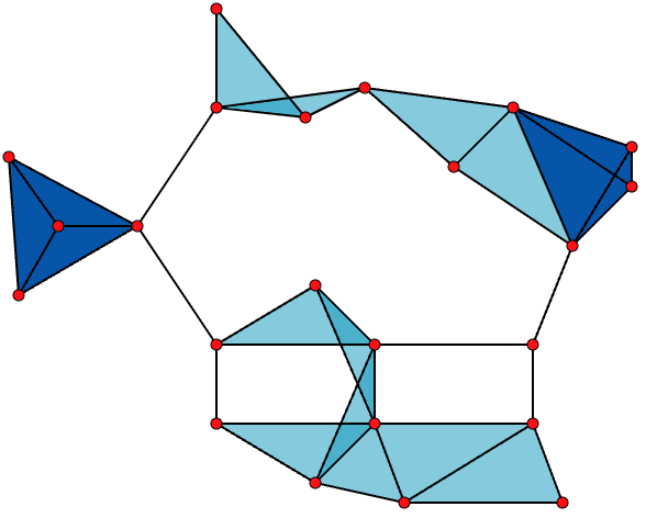
The above is a graph with

• 23 x 1-vertex cliques (the vertices),
• 42 x 2-vertex cliques (the edges),
• 19 x 3-vertex (cliques) (light and dark blue triangles), and
• 2 x 4-vertex cliques (dark blue areas).

The 11 light blue triangles form maximal cliques. The two dark blue 4-cliques are both maximal and minimal, and the clique number of the graph is 4.

We won't need all of the detail from the Wiki example above, but it helps with being able to immediately understand some terminology.

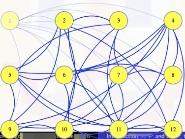
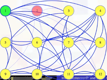
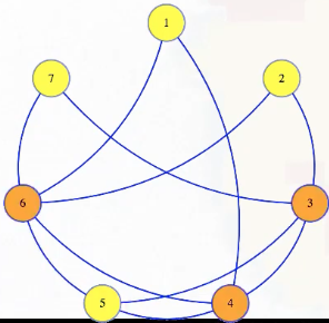
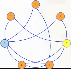
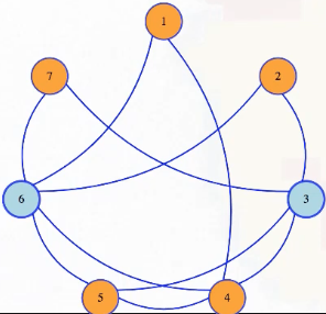
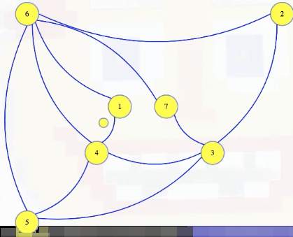
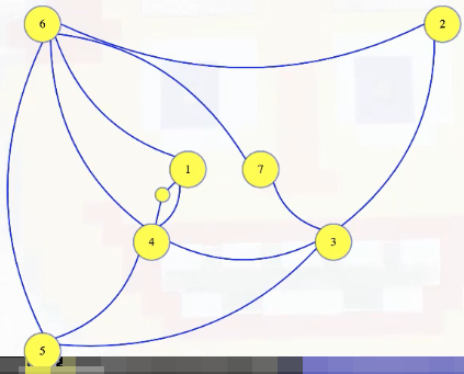
For this post, we'll consider the following graph:

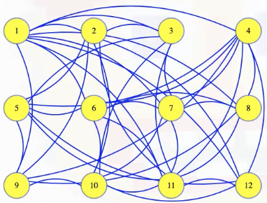
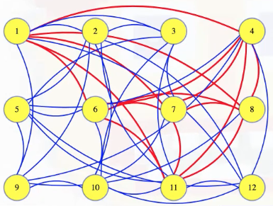
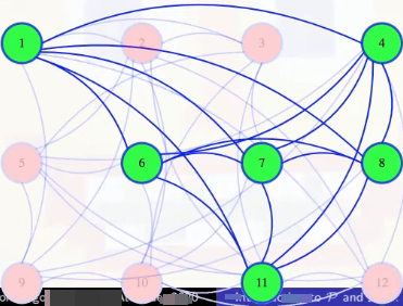
The size 6 clique hidden above is hard to detect at first, but we'll color it to make it clear what clique we're talking about:

An easy clique question

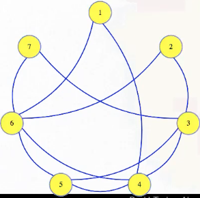
Above, we can see just how difficult it might be to manually just look at a graph and determine whether or not there's a clique of a certain size. Suppose, however, someone tells us that some set of vertices in the graph defines a clique:

It's easy to verify: we can go through each pair of vertices in the set to check that there's an edge between them (and stop if we ever encounter a pair that isn't connected):

How long this takes might depend on what format the graph is in, but it shouldn't take more than $O(|V|^2)$ time, so polynomial in the size of the input.

Let's recap:

• Clique verification: given graph $G = (V, E)$ and $C\subseteq V$, is $C$ a clique in $G$?

• Check vertices, pair by pair, for edges:

  • $O(|C|^2)$ for adjacency matrix.
  • $O(|C|^2|V|)$ for adjacency list.
  • Improve to $O(|C||V|)$: Sort $C$ and each adjacency list for vertex in $C$ with linear time sort. Then a linear pass through each list can check edges to all vertices in $C$.)

  Consider either case as $O(|V|^2)$.

P definition

This brings us to the complexity class, $\mathcal{P}$:

If a decision (yes/no) problem of input size $n$ can be solved in $O(n^c)$ time for any constant, $c$, then the problem is in the complexity class $\mathcal{P}$ ($\mathcal{P}\text{olynomial}$).

Wiki again gives us a slightly more precise definition that may be helpful:

In computational complexity theory, P, also known as PTIME or DTIME($n^{O(1)}$), is a fundamental complexity class. It contains all decision problems that can be solved by a deterministic Turing machine using a polynomial amount of computation time, or polynomial time.

Problems fall into the $\mathcal{P}$ complexity class if they are decision problems (i.e., yes/no problems) that can be solved in polynomial time.

Asymptotic notation ignores constant multipliers so we can give a set of problems that can be solved in, let's say, $O(n^2)$ runtime regardless of the coefficient. This, however, is like asymptotic notation on steroids: we're allowed to ignore constant exponents; that is, this idea of $\mathcal{P}$ as a complexity class goes further than regular asymptotic notation, ignoring constant exponents, so it catches all polynomials of any fixed degree.

Roughly speaking, for a real-world word problems that come up, if we can find a polynomial time algorithm to solve them, then the thought is that those problems can be solved efficiently. Of course, algorithms that are $n^{100}$ in runtime are polynomial but not efficient, but those don't come up so much.

Because we can solve the clique verification problem in polynomial time, and because it's a decision problem, we see the verification problem is in $\mathcal{P}$:

$$\text{Clique Verification}\in\mathcal{P}$$

A harder clique question

The clique problem gets harder if we are just given a graph and asked if it has a clique of a given size without being told what the clique is:

Clique problem: Give $k\geq 0$, $G = (V, E)$, does $G$ have a clique of size $k$?

We could just check each possible subset of the right size. If we fix the size, and ask how the runtime of that changes as the graph grows, it's polynomial, though for not very practical for large sizes. But if we let the size also grow with the runtime, then it isn't polynomial anymore. That's not a problem for a tiny graph, but if, say, we want to check all 25 subsets in a small graph with 50 vertices? There are a lot of possible subsets. We're not going to want to wait for it.

Let's recap:

• Clique problem: Give $k\geq 0$, $G = (V, E)$, does $G$ have a clique of size $k$?
• Idea: check each size $k$ subset of $V$?
  • Fixed $k$: try to verify each of $\binom{|V|}{k}$ subsets, $O(|V|^{k+2})$ each, $O(|V|^{k+2})$.
  • If $k=|V|/2$? Then $\binom{|V|}{2} = \Theta(2^{|V|}/\sqrt{|V|})$, not polynomial (Stirling's approximation).
    • $|V| = 12$ gives 924 subgraphs
    • $|V| = 50$ gives 126,410,606,437,752 subgraphs

NP definition

The clique problem discussed above is in a complexity class called $\mathcal{NP}$, short for non-deterministic polynomial. That name comes from the original way the class was defined, but we'll use a different definition here that defines the same class:

If, for all instances of a decision problem of input size $n$, there exists a certificate/proof that can be used to prove it in $O(n^c)$ time for any constant $c$, then the problem is in the complexity class $\mathcal{NP}$ ($\mathcal{N}\text{on-deterministic}$ $\mathcal{P}\text{olynomial}$)

The Wiki excerpt on the NP complexity class is informative:

In computational complexity theory, NP (nondeterministic polynomial time) is a complexity class used to classify decision problems. NP is the set of decision problems for which the problem instances, where the answer is "yes", have proofs verifiable in polynomial time by a deterministic Turing machine, or alternatively the set of problems that can be solved in polynomial time by a nondeterministic Turing machine:

• NP is the set of decision problems solvable in polynomial time by a nondeterministic Turing machine.
• NP is the set of decision problems verifiable in polynomial time by a deterministic Turing machine.

The first definition is the basis for the abbreviation NP: "nondeterministic, polynomial time". These two definitions are equivalent because the algorithm based on the Turing machine consists of two phases, the first of which consists of a guess about the solution, which is generated in a nondeterministic way, while the second phase consists of a deterministic algorithm that verifies whether the guess is a solution to the problem.

It is easy to see that the complexity class P (all problems solvable, deterministically, in polynomial time) is contained in NP (problems where solutions can be verified in polynomial time), because if a problem is solvable in polynomial time, then a solution is also verifiable in polynomial time by simply solving the problem. It is widely believed, but not proven, that P is smaller than NP, in other words, that decision problems exist that cannot be solved in polynomial time even though their solutions can be checked in polynomial time. The hardest problems in NP are called NP-complete problems. An algorithm solving such a problem in polynomial time is also able to solve any other NP problem in polynomial time. If P were in fact equal to NP, then a polynomial-time algorithm would exist for solving NP-complete, and by corollary, all NP problems.

The complexity class NP is related to the complexity class co-NP, for which the answer "no" can be verified in polynomial time. Whether or not NP = co-NP is another outstanding question in complexity theory.

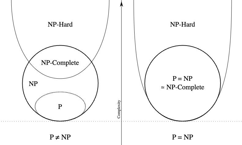
The following is an Euler diagram for P, NP, NP-complete, and NP-hard set of problems:

Under the assumption that P ≠ NP, the existence of problems within NP but outside both P and NP-complete was established by Ladner.

As noted previously, we have $\text{Clique Problem}\in\mathcal{NP}$ ("yes" instances can use the clique itself as a certificate). We already saw that if someone gives us the clique itself as a certificate, then we can verify that it's a clique, but we don't know of any polynomial time algorithms to solve the clique problem.

For instances with a "no" answer, we don't need a proof, but our verification algorithm can't ever be tricked into verifying that a "no" instance is a "yes" instance (i.e., "no" instances don't require a easily verified proof). If we have a decision problem where negative instances have proofs that can be verified in polynomial time, but we don't need a proof for "yes" instances, those problems are in the complexity class co-$\mathcal{NP}$: their complement; that is, if the complement of a problem is in $\mathcal{NP}$, then the problem is in co-$\mathcal{NP}$, and "no" instances will have certificates.

P is a subset of NP

$\mathcal{P}$ is for sure a subset of $\mathcal{NP}$ and co-$\mathcal{NP}$: $\mathcal{P}\subseteq\mathcal{NP}$ and $\mathcal{P}\subseteq\text{co-}\mathcal{NP}$. For problems in $\mathcal{P}$, instances don't need any certificate: in polynomial time, solve any instance, and that verifies if it has a "yes" or "no" answer:

$\mathcal{P}\subseteq\mathcal{NP}$ and $\mathcal{P}\subseteq\text{co-}\mathcal{NP}$ For any instance of a problem in $\mathcal{P}$, an empty certificate is sufficient: in polynomial time, we can solve the problem from scratch to verify that is a "yes" or "no" instance.

Also, remember that saying a problem is in $\mathcal{NP}$ doesn't imply that it's hard — it's a statement of ease. It is a limit on how hard the problem is, but the problem might still be very easy. Everything in $\mathcal{P}$ is also in $\mathcal{NP}$. It would be like if we told someone that, as a professor, we make less than a billion dollars per year. That gives an upper limit on our salary. It's a high limit, but maybe we don't even make half that amount.

Decision vs. optimization problems

Of course, lots of times we're interested in optimization problems, not decision problems. But if we had a way to efficiently solve the decision problem, then we might be able to use that to solve the optimization problem. Let's consider the clique problem again.

Suppose we had a polynomial time black box that could solve CLIQUE (i.e., the clique problem), the decision version, in polynomial time. Could this help us to solve any optimization problem? A simple optimization version might ask what's the size of the largest clique in a graph. We could use the black box in a binary search to find the largest size, or we could just be lazy and just do a linear search.

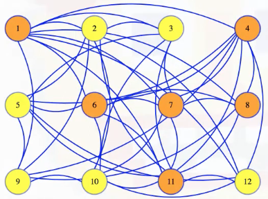
Either way, we run the polynomial time black box a polynomial number of times. So it takes polynomial time to answer. But what if we actually wanted to find a maximum-sized clique? Well, first find what the size of the largest clique is. It's 6 for the graph we first looked at:

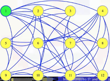
Next, we can go through our vertices, one at a time, to see if they are needed to make a clique of that size. Maybe we make a new graph with the first vertex removed, and we ask if there is still a clique of that maximum size in the new graph. In the case below, there isn't:

So we made a mistake. That first vertex is needed in our clique. So we go back to the previous graph, marking that the first vertex is definitely in the clique:

And then we try removing the second vertex next. The black box tells us that there is still a clique of size 6 without that vertex. There might also be a size 6 clique that includes vertex 2, but whether or not there is one, we know there is one without it (we should try to find one of those):

Above, since there's a size 6 clique that doesn't include vertex 2, not necessarily unique, we permanently exile vertex 2 and continue on. In general, we temporarily delete vertices, and if the resulting graph still has a clique of the maximum size, then we make that deletion permanent; otherwise, we bring the vertex and its edges back into the graph, marking that it will be in our clique

When we keep 11 at the end of the animation above, we now have 6 vertices marked. They must form a size 6 clique, but we could also just continue with the algorithm, which would tell us to toss vertex 12:

We end up running that black box a linear number of times, and it takes polynomial time each, so that gives us a slightly larger polynomial time algorithm to solve the optimization problem.

Let's recap:

• Suppose we have a black box to solve CLIQUE in polynomial time.
• Can we use it to find the size of the largest clique in polynomial time?
• Possible approaches:

  • Binary search to find largest $k$ such that $G$ has a clique of size $k$.

  • Linear search to find largest $k$ such that $G$ has a clique of size $k$:

    LargestCliqueSize(G = (V, E)) {
        k = |V|
        while (!Clique(G, k))
            k--
        return k
    }
• Can we use the black box to find a clique of maximum size in polynomial time?
  • Find $k$, the size of the maximum-sized clique in the graph.
  • Remove a vertex from the graph, check if a size $k$ clique still remains.
    • If not, we needed that vertex. Put it back, and mark it as part of our clique.
    • If so, we don't need that vertex. Discard it forever.
  • Do that until we are left with just a clique of size $k$.
  • $O(|V|)$ total calls to CLIQUE will take polynomial time.

Open questions

There are lots of open questions about complexity classes, and the granddaddy of them all is whether or not $\mathcal{P}$ is equal to $\mathcal{NP}$:

$$\mathcal{P}\stackrel{?}{=}\mathcal{NP}$$

The general consensus is that $\mathcal{P}\neq\mathcal{NP}$, but that hasn't been proved. If they aren't equal, then there are still other related questions that might still need to be answered like whether $\mathcal{NP}$ equals $\text{co-}\mathcal{NP}$, and if they aren't equal, then does $\mathcal{P}$ equal their intersection?

More concisely in symbols:

• $\mathcal{P} = \mathcal{NP}$?
• $\mathcal{NP} = \text{co-}\mathcal{NP}$?
• $\mathcal{P} = \mathcal{NP}\cap\text{co-}\mathcal{NP}$?

NP-complete reductions - clique, independent set, vertex cover, and dominating set

Independent set definition

Let's start by defining the independent set problem. To do that, we need to have a working definition of what an independent set actually is:

Independent set: Within an undirected graph $G = (V, E)$, an independent set is a set of vertices $X\subseteq V$ such that $E$ contains no edges between two vertices in $X$.

Simply put, an independent set is basically a set of vertices with no edges between them:

If edges model dependencies of vertices, then everything in the independent set is pairwise independent:

The independent set problem asks if there is an independent set of a given size in a graph.:

Independent set problem: Given $k_i$, $G_i = (V_i, E_i)$, does $G_i$ have an independent set of size $k_i$?

The independent set problem is in $\mathcal{NP}$: $\text{IndSet}\in\mathcal{NP}$. If we give the independent set of size $k$ as a certificate, then we can write a polynomial time algorithm to verify that the graph doesn't have any edges between any pair of vertices in that set. It's in $\mathcal{NP}$, but we don't know how to solve it in polynomial time without a certificate. So we don't know if it is in $\mathcal{P}$.

Reducing independent set to/from clique

But suppose we could solve the clique problem in polynomial time. Could we somehow use that to solve the independent set problem quickly? That is,

• Given a black box that solves:
  • Clique: Given $k_c$, $G_c = (V_c, E_c)$, does $G_c$ have a clique of size $k_c$?
• how can we use this to solve:
  • IndSet: Given $k_i$, $G_i = (V_i, E_i)$, does $G_i$ have an independent set of size $k_i$?

Well, if we have a graph with a size $k$ independent set (e.g., k = 4 with vertices 1, 2, 5, 7 in the graph above), and then we take the complement of that graph, which has all of the missing edges but doesn't have any of the edges from the original graph, then that complement graph will have every edge between vertices in the original graph's independent set. The complement of an independent set is a clique:

Symbolically, we're letting $G_c = \overline{G_i}$, $k_c = k_i$, and we're saying that $G_i$ has an independent set of size $k_i$ if and only if $G_c$ has a clique of size $k_c$>

There are a few different types of reductions, but this is the type we are going to care about here. This is a reduction of IndSet to Clique: given an instance of IndSet, run a polynomial time program to create an instance of Clique such that the IndSet instance is true if and only if the Clique instance is true (i.e., the original problem and the new reduction problem have the same "yes"/"no" answer). We symbolize that as follows:

$$\text{IndSet}\leq_p \text{Clique}$$

The "$\leq$" sign implies that the independent set problem isn't harder than the clique problem, because the clique problem can be used to solve it. The $p$ in $\leq_p$ denotes that we are allowed to take polynomial time to transform an instance of one problem into an instance of the other.

One that thing that this reduction has that is a bit unusual is that it works both ways: the same transformation that changes the independent set instance into a clique instance also reduces a clique instance into an independent set instance, because the complement of a clique is an independent set.

Vertex cover definition

In a graph, a vertex covers the edges that it's a part of. A vertex cover is a set of vertices that covers all of the edges in a graph:

Vertex cover: Within a graph, $G = (V, E)$, a vertex cover is a set of vertices $X\subseteq Y$ such that for each $e = (u, v)\in E$, $u\in X$ or $v\in X$ (or both).

We can see this in our sample graph:

The vertex cover problem asks if a graph has a vertex cover of a given size:

Vertex cover problem: Given $k\geq 0$, $G = (V, E)$, does $G$ have a vertex cover of size $k$?

Note that it's harder to find a small vertex cover while it's harder to find large cliques and large independent sets. But still, the vertex cover problem is in $\mathcal{NP}$: if somebody gives us a cover as a certificate, then in polynomial time we can mark edges for each vertex in that cover, and then verify if all edges from the graph are marked:

Reducing independent set to/from vertex cover

We can reduce independent set to vertex cover.

• Given a black box that solves:
  • VertCover: Given $k_v$, $G_v=(V_v, E_v)$, does $G_v$ has a vertex cover of size $k_v$?
• How can we use it to solve:
  • IndSet: Given $k_i$, $G_i = (V_i, E_i)$, does $G_i$ have an independent set of size $k_i$?

Note that, in a graph, no edges go between two vertices of an independent set, which means that every edge either goes from the independent set to something not in the set or between vertices not in the set. Either way, every edge has at least one vertex not in the independent set; the vertices not in the independent set form a vertex cover:

Symbolically, let $G_v = G_i$, $k_v = |V_i| - k_i$. Then $G_i$ has an independent set of size $k$ if and only if $G_v$ has a vertex cover of size $k_v$.

In the animation above, we have a size 4 independent set in the graph with 7 vertices if and only if there is a vertex cover of size 7 - 4 = 3.

This reduction also happens to work both ways.

Reduction compositions

Now we know that clique reduces to independent set, and independent set reduces to vertex cover. These reductions are transitive:

$$\text{Clique}\leq_p\text{IndSet} \quad\text{and}\quad \text{IndSet}\leq_p\text{VertCov} \quad\text{so}\quad \text{Clique}\leq_p\text{VertCov}$$

Taking the composite of two polynomial time reductions gives us another polynomial time reduction: Given an input for Clique, reduce it to an input for IndSet. Then, reduce that input for IndSet to an input for VertCov. Each reduction takes polynomial time, and the composite of polynomials is a polynomial, so the total reduction also takes polynomial time.

In the case above, to reduce Clique to IndSet, we took the complement of the graph, and then to go from independent set to vertex cover, we changed the size we were looking for. Doing both of those things gives the reduction from clique to vertex cover.

NP-hard and NP-complete definitions

We're now ready to define some new complexity classes. Because independent set reduces to clique, in some sense we say that clique is at least as hard as independent set.

Now suppose we have some problem X that is at least as hard as any $\mathcal{NP}$ problem. That is, for any problem in $\mathcal{NP}$, we can reduce it to problem X, so X is as hard as any of them. We say that X is $\mathcal{NP}$-Hard.

For decision problem $X$, if for every problem $x\in\mathcal{NP}$, $x\leq_p X$, $X$ is $\mathcal{NP}$-Hard.

Unlike $\mathcal{NP}$, the $\mathcal{NP}$-Hard complexity class is a statement of difficulty, not ease. Clique is $\mathcal{NP}$-Hard.

So now we have a statement of ease for clique and also a statement of difficulty. If a problem is in both of these complexity classes, then we say it is $\mathcal{NP}$-Complete. So clique is $\mathcal{NP}$-Complete:

If $X\in\mathcal{NP}$ and $X\in\mathcal{NP}$-Hard, then $X\in\mathcal{NP}$-Complete.

Proving additional problems are NP-hard

Even though we're not going to prove that clique is $\mathcal{NP}$-Hard, if we accept that it is, then it becomes much easier to prove that other problems are $\mathcal{NP}$-Hard too.

We already know independent set is in $\mathcal{NP}$, and that clique reduces to independent set, and we're taking it as a given that clique is $\mathcal{NP}$-Hard. Intuitively, if independent set is at least as hard as clique, and clique is $\mathcal{NP}$-Hard, then so is independent set.

More formally, we know for any problem in $\mathcal{NP}$, it reduces to clique, and we know that clique reduces to independent set, so we can take the composite of those reductions to reduce any problem in $\mathcal{NP}$ to independent set in polynomial time. That proves independent set is $\mathcal{NP}$-Hard, and so it's $\mathcal{NP}$-Complete.

Similarly, we've seen reductions from clique and independent set to vertex cover, so that is also $\mathcal{NP}$-Hard and $\mathcal{NP}$-Complete.

In summary:

• $\text{IndSet}\in\mathcal{NP}$ (previously outlined)
• $\text{Clique}\leq_p\text{IndSet}$ (previously outlined)
• $\text{Clique}\in\mathcal{NP}$-Hard (not proven but accepted)
• $\text{IndSet}\in\mathcal{NP}$-Hard:
  • for all $x\in\mathcal{NP}$, $x\leq_p\text{Clique}$ (definition of $\text{Clique}\in\mathcal{NP}$-Hard)
  • for each $x\in\mathcal{NP}$, $x\leq_p\text{Clique}$ and $\text{Clique}\leq_p\text{IndSet}$, so $x\leq_p\text{IndSet}$.
• $\text{IndSet}\in\mathcal{NP}$-Complete.

One $\mathcal{NP}$-Hard problem reduced to another problem proves it's also in $\mathcal{NP}$-Hard. So, $\text{VertCov}$ is $\mathcal{NP}$-Complete too (by previous reductions).

This covers the basics of the definitions, but it's a bit misleading to only show reductions that work in both directions because those are actually pretty rare. So we'll show one more that does not work in both directions.

Dominating set definition

Dominating set: Within a graph $G = (V, E)$, a dominating set is a set of vertices $X\subseteq V$ such that, for each $v\in V$, $v$ or something adjacent to $v$ is in $X$ (or both).

Dominating set problem: Given $k_d$, $G_d = (V_d, E_d)$, does $G_d$ have a dominating set of size $k_d$?

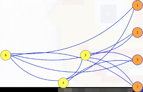
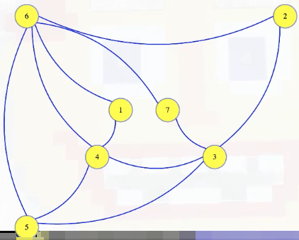
In a graph, a vertex dominates itself and all adjacent vertices. In the graph below, vertex 6 dominates everything except 3:

A dominating set is a set of vertices that dominate all vertices in a graph, and we can ask if a graph has a dominating set of a given size. That question is in $\mathcal{NP}$: if somebody suggests a dominating set to us as a certificate, then mark each vertex and everything adjacent to it, and then check that all vertices of the graph are marked.

So above, if we add vertex 3 to vertex 6, then we could verify that those two vertices are a dominating set:

It would only take time linear in the input size to check, for adjacency list or adjacency matrix format. So, dominating set is in $\mathcal{NP}$. Now we want to find a reduction from vertex cover to dominating set.

• Given a black box that solves:
  • DomSet: Given $k_d$, $G_d = (V_d, E_d)$, does $G_d$ have a dominating set of size $k_d$?
• how can we use this to solve:
  • VertCover: Given $k_v$, $G_v = (V_v, E_v)$, does $G_v$ have a vertex cover of size $k_v$? (for whatever inputs we give it)

Reducing vertex cover to dominating set

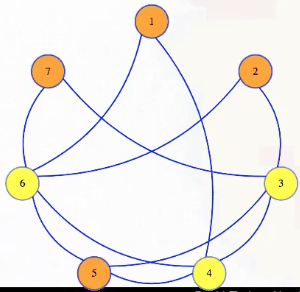
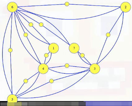
This will be a bit more complex than previous reductions. So, we're given some instance of vertex cover, maybe this graph:

We're asked if it has a vertex cover of size 3. We need to transform this into a dominating set instance, and we'll create a pretty different looking graph for that for visibility:

Consider the edge from vertex 1 to 4. For that edge, let's create a brand new vertex. We won't label it, and we'll make it small:

Now let's give it two edges, to the two vertices of that original graph:

Those will be part of our dominating set instance graph. It will have all of the original vertices and edges, plus one of these little vertices and two edges for every edge in the vertex cover instance:

We're wanting to show $\text{VertCov}\leq_p\text{DomSet}$:

• Given $G_v$, create $G_d$: it contains each edge and vertex of $G_v$, plus a vertex and two edges per edge in $G_v$ as shown. $k_d = k_v$
• $G_v$ has a vertex cover of size $k$ if and only if $G_d$ has a dominating set of size $k_d$.

Let's think about these new vertices in the new dominating set graph. First, each one only dominates itself and the two vertices that created it:

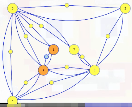
So that first vertex we added dominates only itself, 1, and 4, as shown above. Meanwhile, both 1 and 4 have to dominate those same three vertices because, by construction, each is adjacency to the other two. But, 1 and 4 might also be adjacent to other stuff, so each might dominate more, each dominates a superset of the stuff dominated by the new vertex. Because of that, we can be sure that there is a minimum-sized dominating set that only contains original vertices, because we can always replace a new vertex with one of the originals. But notice, if we have a vertex that dominates a new vertex, then it covers the original edge that spawned that new vertex.

A set of original vertices that dominate all of the new vertices, like 3, 4, and 6, will also dominate all of the other original vertices, but they also must cover all of the edges taken directly from the original graph. They will cover at least half of the new edges too, but we don't really care about those: we are looking for a vertex cover in the original graph. There is a minimum-sized dominating set in the new graph that doesn't include any of the new vertices, and those vertices form a vertex cover in the original graph.

If there was a smaller vertex cover in the original graph, then those vertices would make a smaller dominating set in the new graph. So, the size of the smallest dominating set in the new graph will be the size of the smallest vertex cover in the original. One small technicality: we assume there aren't any singleton vertices with no edges in the original graph. Those vertices can be ignored in the vertex cover graph. They don't cover anything, so we shouldn't include them in our dominating set graph. A singleton in a dominating set instance must be in the solution — nothing else dominates it.

Everything above gives us a reduction from vertex cover to dominating set, so dominating set is $\mathcal{NP}$-Hard and $\mathcal{NP}$-Complete.

To recap what we've seen so far:

• A new vertex dominates: itself and vertices of the edge that spawned it.
• Either corresponding original vertex dominates the same set and maybe more.
• There exists a dominating set of minimum size with only "original" vertices.
• An original vertex that dominates new vertex x covers the edge that spawned x.
• Original vertices that dominate all new ones cover all original edges.
• No smaller cover in $G_v$ exists: it would be a dominating set in $G_d$. (We assume no singleton vertices in $G_v$; they can be ignored for the cover.)
• So, $\text{DomSet}\in\mathcal{NP}$-Hard and $\text{DomSet}\in\mathcal{NP}$-Complete.

But this reduction doesn't reverse itself. Unlike the previous reductions we saw, if we tried to apply the transformation to a dominating set graph, it doesn't transform it to a helpful vertex cover instance; that is, applying the same transformation to an arbitrary instance of DomSet does not reduce it to an instance of VertCover.

Given an arbitrary graph, we can't "undo" the transformation that went from vertex cover to dominating set: a graph like this one doesn't have those little triangle vertices and edges to remove to get a corresponding vertex cover problem. But there has to be a reduction in the other direction because dominating set is in $\mathcal{NP}$, and vertex cover is in $\mathcal{NP}$-Hard, so by the definition of $\mathcal{NP}$-Hard, there must be some reduction from dominating set to vertex cover.

One could make an entire course out of studying approximation algorithms, polynomial time algorithms that don't perfectly solve optimization versions of $\mathcal{NP}$-Complete problems, but that can guarantee that their performance isn't too bad.

---