Minimum spanning trees (with attitude)

This post explores minimum spanning trees (MSTs), specifically the cut property used by most MST algorithms, and then the most popular MST algorithms themselves: Kruskal, Boruvka, and Prim.

Attribution

The notes below come from the Algorithms with Attitude YouTube channel, specifically the Graphs: Basics playlist comprised of the following videos: Introduction to Minimum Spanning Trees, Kruskal's Minimum Spanning Tree Algorithm, Boruvka's Minimum Spanning Tree Algorithm, and Prim's Minimum Spanning Tree Algorithm.

There are several sections in this post, accessible in the table of contents on the right, but most of the sections have been listed below for ease of reference and navigation.

• Introduction to minimum spanning trees (MSTs)
  • Problem definition
  • Assumptions
  • Term definitions
  • Cut crossing theorem
  • Unique spanning tree theorem
  • Cycle theorem
  • Generic algorithm
• Kruskal's algorithm
  • Idea
  • Outline
  • Tracking trees
  • Performance
• Boruvka's algorithm
  • Idea
  • Outline
  • Example (first phase)
  • Algorithm
  • Example (second phase)
  • Example (third phase)
  • Analysis
  • Optimizations
• Prim's algorithm
  • Idea
  • Outline
  • Running example (first vertex)
  • Running example (second vertex)
  • Algorithm
  • Running example (vertices 3-5)
  • Running example (sixth vertex)
  • Running example (seventh vertex)
  • Running example (remaining graph)
  • Comparison to Dijkstra's
  • Analysis
• Interactive examples

Interactive examples

The interactive examples are arguably the most valuable feature of this post. They make it possible to test out each algorithm on the same graph and see the resultant output. Confirm how the algorithms work for yourself, and then tweak the code to experiment.

It's also worth noting that the algorithm implementations used for the examples do not assume that edge weights are distinct. This makes the algorithms more broadly applicable and useful.

Introduction to minimum spanning trees (MSTs)

In this section, we'll introduce the definition of minimum spanning trees (MSTs) and the common ideas used in several different MST algorithms, namely Kruskal's algorithm, Borůvka's algorithm, and Prim's algorithm.

Problem definition

Let's start by defining the problem we're going to try to solve.

We're given a weighted, undirected graph. Our goal is to find the subset of the edges that connect everything in the graph, they span the graph, they have no cycle so they form a spanning tree, and the sum of their weights is minimized. We can express all of this more formally in the following way.

• Given: A weighted, undirected graph $G = (V, E)$
• Find: A set $T\subseteq E$ such that
  • $T$ connects all vertices of $V$ into one component (it spans the graph)
  • $T$ has no cycles (with the condition above, this means $T$ is a spanning tree)
  • Over all spanning trees (there may be several), the sum of edge weights in $T$ is minimized

For example, the graph

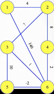
has the following as an MST (for some graphs, there may be more than one MST):

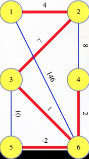
We can imagine wanting to find an MST if we're trying to run electrical wire to connect a system (modeled as a graph) and want to minimize wire length. Indeed, for Borůvka's algorithm, the first known MST algorithm:

It was first published in 1926 by Otakar Borůvka as a method of constructing an efficient electricity network for Moravia.

Assumptions

We're going to assume the graph on which we want to find an MST is connected; otherwise, there is no spanning tree to find (i.e., a spanning tree does not exist). If we assume the edge weights are distinct, then we can prove that this forces the graph to have a unique MST — without this assumption, the algorithms still find MSTs, but the proofs are a bit more complex (because the MST is no longer necessarily unique). That's why texts like CLRS [21] talk about safe edges instead of MST edges. If everybody can agree on any arbitrary but consistent way to break ties for edge weights (e.g., order the vertices, earlier vertex is first tiebreaker, later vertex is second tiebreaker), then the proofs we will show still apply.

Let's recap the assumptions above:

• $G$ is connected (otherwise no spanning trees exist)
• Edge weights are distinct (useful as a simplification step but not great when actually trying to use the algorithms)
• Arbitrarily order the edges and use that order to break ties (e.g., order the vertices, earlier vertex is first tiebreaker, later vertex is second tiebreaker)

Distinct edge weights let us simplify our language. We can talk freely about discarding an edge because it's not in the unique MST. That's simpler than discarding an edge because without it there still exists another MST that also matches whatever other choices we've made up to that point. It basically guarantees consistency and economy of expression when it comes to describing the processes used for the different algorithms to identify an MST.

Term definitions

We'll use the following graph to illustrate a variety of different points throughout the rest of this post (we'll see other graphs, including graphs with non-distinct edge weights, when we get to the interactive examples):

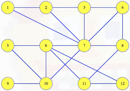
Let's now map out a few definitions to help unify our language. A cut in a graph is a partitioning of the vertices into two disjoint sets. For example, we can imagine partitioning the graph above, where vertices 4, 6, 11 and 12 get placed into one set and all the other vertices in another set:

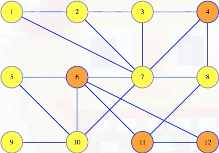
There's nothing special about how the vertices are arranged. We can move them around to make the cut a bit clearer (note that we're just manually repositioning the vertices, but the underlying structure/definition of the graph does not change):

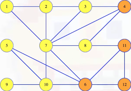
It now becomes a little easier to see which edges cross the cut:

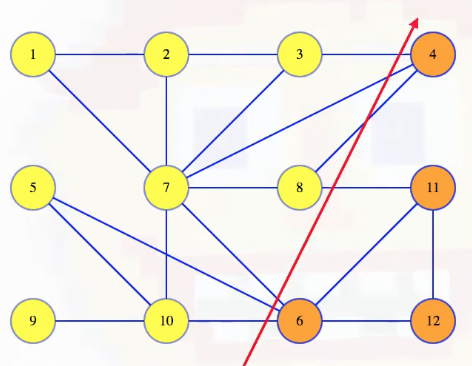
Our main theorem is that the minimum weight edge crossing any cut is in the MST:

Cut Crossing Theorem$\quad$ The edge with minimum weight crossing any cut is in the MST.

Let's recap the definitions discussed above:

• A cut of a graph $G = (V, E)$ partitions the vertices into two disjoint sets, $S\subseteq V$ and $V - S$.
• An edge crosses the cut if it has one vertex in $S$ and the other in $V - S$.
• Cut crossing theorem: The edge with minimum weight crossing any cut is in the MST.

Cut crossing theorem

What's the minimum weight edge crossing the cut pictured above? We don't know yet because edge weights haven't been assigned! But, for right now, let's suppose the minimum weight edge is the edge connecting vertices 3 and 4:

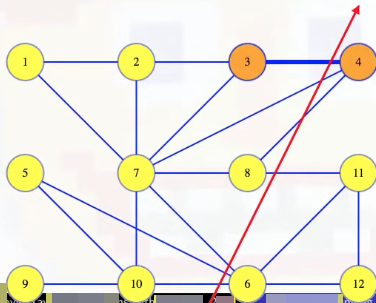
How could we prove this? By contradiction. If that edge isn't in the MST, then the MST is something else. Maybe it's the red edges pictured below:

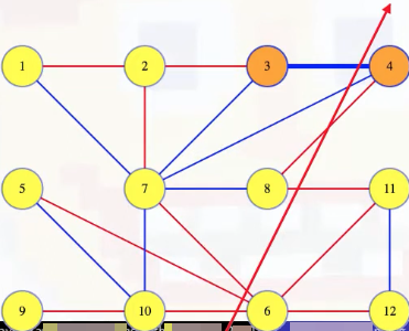
Note that if we add the (3, 4) edge to the tree pictured above, it has to complete a cycle with some of the edges of the tree because 3 and 4 were already connected by some path in the tree:

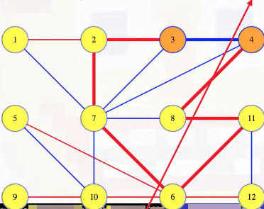
But if we follow the tree's path from 3 to 4, then it has to cross the cut somewhere because the path starts on 3's side of the partition and ends on 4's side of the partition.

More generally, any cycle must cross any cut an even number of times because it ends where it starts. The edge (3, 4) crosses the cut once so the other edges of that cycle, all from the tree, have to cross the cut an odd number of times (at least once). If the cycle crosses the cut between 8 and 4, then that edge must weigh more than the (3, 4) edge, which was the minimum weight edge crossing the cut. But suppose we now delete the (8, 4) edge from the MST and add in the (3, 4) edge:

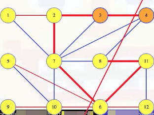
We get a new spanning tree:

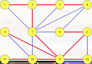
And its weight is less than the tree we had, which was supposedly an MST. The (3, 4) edge, being the minimum weight edge to cross a cut, and not being in the MST, gave us a contradiction.

Let's recap the contradiction we just walked through:

• Suppose the minimum weight edge over some cut is not in the MST. We chose the edge (3, 4) for the cut between $S = \{4,6,11,12\}$ and $V - S$.
• The edge, plus some edges in the MST, form a cycle (e.g., $(3, 2, 7, 6, 11, 8, 4, 3)$).
• Lemma: Any cycle must cross the cut an even number of times (we have to end up back where we started so we either don't cross the cut at all or we cross it and have to return, cross it and have to return, etc., resulting in crossing the cut an even number of times).
• Removing other crossing edge and adding (3, 4) to the tree lowers its cost.
• So, MST didn't have minimum weight. Contradiction.

There's a specific way we're going to use the cut crossing theorem. Each cut will be between some known subtree of the MST and the rest of the graph; that is, for some $T_i = (V_i, E_i)$, a subtree of the MST of $G$, we will consider the minimum edge weight cross the $V_i$, $V - V_i$ cut. Going from the subtree to the rest of the graph defines the cut.

The way we've worded the cut crossing theorem reflects the fact that we're assuming edge weights are distinct:

The edge with minimum weight crossing any cut is in the MST.

That is, our theorem assumes that distinct weights force a unique minimum spanning tree.

Unique spanning tree theorem

Let's now prove that our theorem actually guarantees a unique minimum spanning tree when we're given a connected graph with distinct edge weights. We'll state this as a theorem itself:

Unique Spanning Tree Theorem$\quad$ If $G$ has distinct edge weights, then $G$ has a unique minimum spanning tree.

Suppose we have the following MST shown in red:

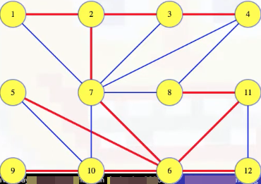
Grab an arbitrary edge such as (7, 6), and ask if it needs to be in the MST. Removing the edge from the tree breaks it into two disjoint sets of vertices, which defines a cut on $G$:

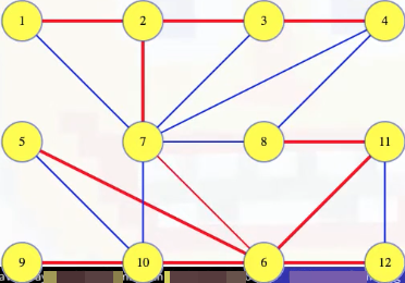
We can see this a bit more clearly if we shift the vertices and draw the cut as a line:

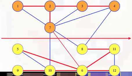
If (7, 6) is the minimum weight edge crossing that cut, then it has to be in any MST by the proof of the cut crossing theorem in the previous section. If some other edge crossing the cut weighs less, like the edge (4, 8), then adding that edge to the remaining edges from our MST gives a new spanning tree with a lower weight than our first tree. The first tree was supposedly an MST so that's a contradiction. So if the (7, 6) edge is in the MST, then it must be the minimum weight edge crossing that cut. So it's definitely in any MST (following the proof of the cut crossing theorem).

This is true for every edge in our MST. Removing an edge from the MST defines a cut on $G$, and the edge must have a minimum weight crossing that cut. So it has to be in any MST. If each edge in the MST shown above has to be in any MST, then the tree is unique. With distinct edge weights, the minimum weight edge crossing any cut is in the MST, and any edge in the MST is the minimum weight edge crossing the cut it defines on $G$ with its tree.

That's a lot. Let's recap again:

• Given an MST, does an arbitrary edge (e.g., (7, 6) in our example) need to be in the tree?
• Removing the edge from the tree breaks it into two, defining a cut on $G$.
• If the edge has the minimum weight crossing that cut, then it is in the MST.
• If another edge crossing the cut weighs less (e.g., (8, 4) in our example), then that edge can reconnect the tree halves for a lower weight spanning tree. Contradiction.
• This argument applies for every edge in the MST. Each edge is required.

Cycle theorem

Just one more theorem:

Cycle Theorem$\quad$ The maximum weight edge in any cycle is not in the minimum spanning tree.

Suppose we have a cycle from the graph:

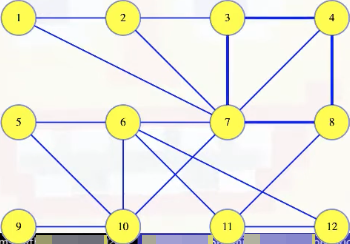
The edge with maximum weight in the cycle cannot be in the MST. Why? The proof will look much like the previous ones (i.e., by contradiction).

Imagine that the edge between 3 and 4 has the maximum weight in the cycle pictured above (i.e., (3, 4, 8, 7, 3)) and that the edge (3, 4) is in the MST:

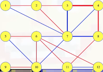
Like in our unique spanning tree proof, removing the edge from the tree defines a cut on $G$:

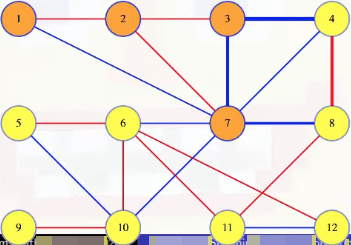
If we're keen on seeing the actual cut, then we can draw a less linear looking cut to capture this:

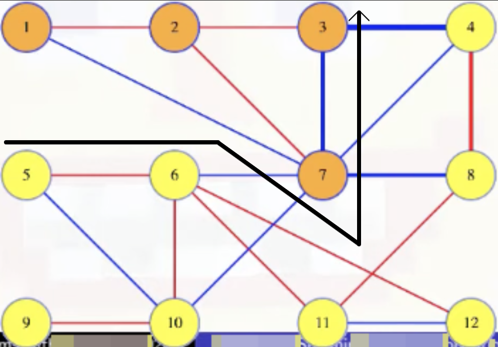
Like in our cut crossing proof, any cycle must cross the cut an even number of times. So besides the (3, 4) edge there must be at least one other edge in the cycle that crosses the cut. Like the edge between 7 and 8. But the (3, 4) edge was the maximum weighted edge from the cycle, which means the (7, 8) edge must weigh less. Let's add the (7, 8) edge to the remaining edges from the MST:

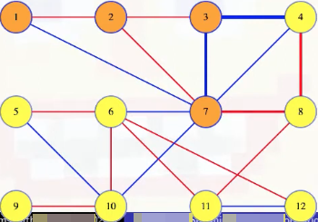
This reconnects the tree to get a cheaper spanning tree than the original MST. This contradicts our assertion that the original MST contained the heaviest edge in the cycle.

Let's recap everything discussed above:

• Assume the MST contains the maximum weight edge from some cycle in the graph (e.g., edge (3, 4) in the example we considered, which is part of the cycle (3, 4, 8, 7, 3)).
• Removing the edge from the tree breaks it into two, defining a cut on $G$.
• The cycle must cross this newly induced cut an even number of times. At least one edge from the cycle besides (3, 4) must cross the cut (e.g., (7, 8), as discussed above).
• Reconnect the tree halves with the lower weight edge, decreasing the tree weight. Contradiction.

Generic algorithm

Now that we're done with the theorems, we can start with the algorithms. Abstractly, each algorithm will keep track of a bunch of trees, each of which is a subtree of the MST. All of those trees combined will include each vertex in the graph once — they make a spanning forest. By finding minimum weight edges crossing the cut between one of the forest trees and the rest of the graph, the algorithms find minimum spannting tree edges and add them to the forest. Each edge merges two trees into one until there's just one tree left, the minimum spanning tree. To initialize the forest, each vertex is in its own uninteresting tree with no edges. We can be sure that each of those single vertices are subtrees of the minimum spanning tree to start.

Different algorithms use different strategies to consider edges in different orders and track trees differently. So that's where the generic algorithm described above ends and where each of the individual algorithms begins.

To recap the generic algorithm:

• Keep a set of disjoint MST subtrees that span the graph.
• If each tree in the forest is named $T_i = (V_i, E_i)$, then, for any $i$, the minimum weight edge crossing the $V_i$, $V - V_i$ cut is in the MST.
• Add MST edges to the forest, merging two trees into one larger MST subtree.
• When the forest has only one tree, we're done.
• Initialize the forest with singleton vertices.

Kruskal's algorithm

Prerequisite (union-find data structure)

Implementing Kruskal's algorithm efficiently relies on understanding the union-find data structure.

Idea

We want to find MST edges to merge trees in our spanning forest. Kruskal's strategy will be to consider the edges with the smallest weights first. In fact, we'll start by sorting all edges by weight, lowest to highest.

For the graph below, we use integer edge weights, starting from 1, which makes it easier to see their order, but they can be anything:

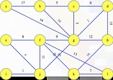
To simplify our proofs, we'll assume edge weights are distinct, but the algorithm works regardless.

We consider edges in order, starting with the lightest edge first. Then, for each, we determine if it's in the MST or not, right then and there. We never wait or change our minds later.

In the pictures that follow, edges that have not yet been looked at are blue, MST edges are red, and discarded edges will be faint.

Suppose we've already gotten to the following step, where the first four edges have been processed:

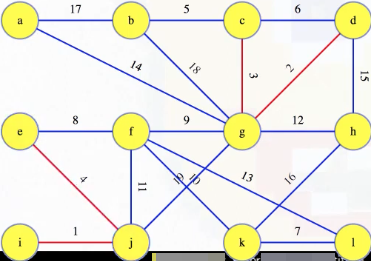
So now we're looking at the edge with edge weight 5. What should we do with it? Do we add it to the MST? The edge connects vertices b and c. If those two vertices are in different trees of the growing forest, then the edge gets added to the MST; otherwise, it's discarded. In this case, we should add the edge (b, c) with weight 5 to the forest, but we should justify this.

Consider either of the trees it connects, say cgd. The claim is that edge 5 is the minimum weight edge crossing the cut from that tree to the rest of the graph. Why? We've already considered all edges with lower weight. At this instant in time, any edge ever added to the forest obviously has both of its vertices in the same tree, and that would be true for any edge we discarded too. It was discarded because its vertices were already in the same tree. So every edge in the graph lighter than this one goes between two vertices previously merged into the same tree. This edge is the lightest of all edges between any of the different trees so it's the lightest edge leaving the cgd tree.

The lightest edge leaving any tree crosses the cut between the tree and the rest of the graph. So, by the cut crossing theorem, this lightest edge is in the MST:

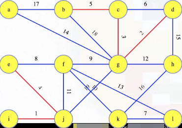
What about when we get to edge 6? It connects two edges already in the same forest tree (i.e., (c, g) and (g, d), which have weights 3 and 2, respectively). How do we justify discarding this edge? c and d are already connected by edges previously added to the forest, and we're taking edges in increasing order so all of those previous edges weight less than this one. So this edge has the maximum weight in a cycle from the graph, and the cycle theorem tells us this edge definitely isn't in the MST. So we can discard it.

Let's recap everything discussed above:

• Sort edges, minimum weight first, and consider edges in order (lowest to highest).
• If an edge's vertices are in different trees of the forest, then add the edge to the forest, merging two forest trees.
  • These are minimum weight edges crossing the cut between either one of their forest trees and the rest of the graph. (Cut Crossing Theorem)
• If an edge falls between different trees in the forest, discard it.
  • These are maximum weight edges in a cycle. (Cycle Theorem)

Outline

We now have the outline of the algorithm and proof that it will find the MST:

Kruskal(G = (V, E)) {
    T = Ø
    L = E, sorted by weight
    for(e = (u, v) in L)
        if(u's tree in the forest != v's tree)
            T = T U {e}
    return T
}

But we left out the detail of how we determine whether or not the vertices of an edge are from the same forest tree or not. We could search the forest, starting from one of the vertices, in order to see if we get to the other, but that's kind of slow. Instead, we'll try to track trees, as they merge, as efficiently as possible.

Tracking trees

Each vertex starts out in its own little tree. We check to see if two vertices are in the same tree or not, and if they aren't, then we add an edge to merge two trees into a bigger one. This is a perfect situation to use the disjoint set union-find data structure:

Context	Union-Find Operation
Each vertex x is alone as its own tree to start.	MakeSet(x)
For edge e = (u, v), check if u's tree != v's tree.	Find(u) != Find(v)
If so, add edge e, combining the trees into one.	Union(u, v)

Kruskal(G = (V, E)) {
    T = Ø
    for(x in V)
        MakeSet(x)                # each vertex starts out in its own set (i.e., as its own tree)
    L = E, sorted by weight
    for(e = (u, v) in L)
        if(Find(u) != Find(v))    # two vertices are in the same tree if they're in the same set (so check if they have the same representative)
            T = T U {e}           # if not, add the edge to the MST
            Union(u, v)           # take the union of these two sets to capture that the trees have been merged
    return T
}

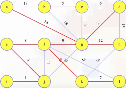
If we run this new algorithm on our original graph, then we end up with the following MST:

It's quite informative if we look at how vertices are combined using the union-find operations. Consider again the state of the graph when we were looking at what to do with edge 5:

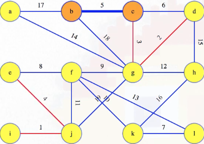
At this point, the union-find setup looks something like the following (note how the tree-like structures from the union-find operations match the growing forest for our MST):

Note that the edges from the union-find structure are not from the graph. For example, consider the state of the graph when we're looking at what to do with edge 15:

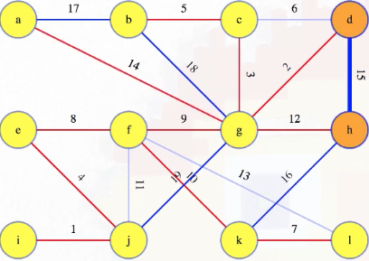
At this point, the union-find structure looks something like the following:

Observe that the edge (j, d) in the union-find structure is not an edge in the graph. The edge in the union-find structure comes about due to path compression.

Once the algorithm concludes, our union-find structure looks as follows:

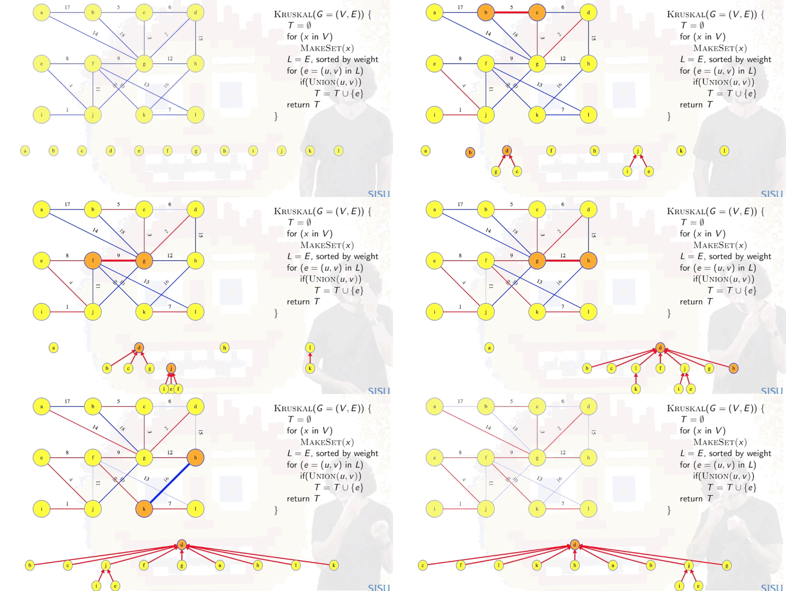
The full animation is provided in the widget below.

Full animation of Kruskal's algorithm

Performance

We could stop once we know we've added $V - 1$ edges. Or not. When we finish, we should check that we have $V - 1$ edges. If we don't, then the graph wasn't connected to begin with. How long does it take?

Kruskal(G = (V, E)) {
    T = Ø
    for(x in V)
        MakeSet(x)                # Θ(|V|)
    L = E, sorted by weight       # O(|E|lg|E|)
    for(e = (u, v) in L)          # O(|E|α(|E|))
        if(Find(u) != Find(v))
            T = T U {e}
            Union(u, v)
    return T
}

Well, the union-find data structure is only marginally super linear so sorting edges by weight will dominate our runtime with a general sort: $\Theta(|E|\lg |E|) = \Theta(|E|\lg|V|)$ worst case runtime, dominated by edge sort. If we have special edge weights that can be sorted in linear time, then the union-set operations dominate our runtime. For all practical purposes, that's linear.

Boruvka's algorithm

Boruvka's algorithm is the oldest MST algorithm, first making an appearance in 1926. It's not in CLRS [21], but it's covered nicely Jeff Erickson's Algorithms book (page 261).

Idea

We start with a forest of single-vertex trees for every vertex in the graph:

Notice that, with distinct edge weights, the minimum weight edge incident on any vertex has to be in the MST. We can justify this with the cut crossing theorem. Each of those edges is a minimum weight edge crossing the cut between the vertex and the rest of the graph. If we calculate all of those edges, then all of them are in the MST.

Boruvka's algorithm generalizes this. It works in phases, where in each phase it figures out what the trees of the growing forest are, finds the minimum edge crossing from each tree to the rest of the graph, and adds all of those edges to the forest.

Let's recap:

• Start with a forest of single vertex "trees" spanning the graph.
• The minimum weight edge incident on any vertex v is in the MST. It's the minimum weight edge crossing the cut between $\{v\}$ and $V - \{v\}$. Boruvka's algorithm generalizes this:
• The minimum weight edge with one vertex in forest tree $T_i$ is in the MST. It's the minimum weight edge crossing the crossing the cut between $T_i$ and $V - T_i$.
• One phase:
  • Mark each $T_i$ tree of the forest.
  • Find the lightest edge leaving each $T_i$.
  • Add all of those edges to the forest.

Outline

Great! This gives us an outline for the whole algorithm:

Boruvka(G = (V, E)) {
    T = Ø
    while(|T| < |V| - 1) {
        figure out which vertices are in each T_i ⊆ T
        find minimum weight edge incident on each T_i (_one_ side only)
        add those edges to T
    }
    return T
}

But we should really fill in some details. How do we know which tree each vertex is in? To start each phase, we'll find the components of the graph made of all the vertices and our minimum spanning tree edges that we've found so far.

We can do this by executing a depth-first search (DFS) on the MST edges we've found so far (it's better to use union-find as in Kruskal's than DFS here):

Boruvka(G = (V, E)) {
    T = Ø
    while(|T| < |V| - 1) {
        initialize each vertex to an unknown component
        discover each T_i by running DFS on (V, T)
            each v discovered by the top level DFS indicates a new component
            initialize each with an infinite weight edge
        find minimum weight edge incident on each T_i (_one_ side only)
        add those edges to T
    }
    return T
}

Example (first phase)

The DFS in the first phase isn't very interesting because we haven't found any MST edges yet (i.e., we have T = Ø on line 5 in the pseudocode above before we start the first phase). So each vertex is discovered by a top-level DFS to be its own component; that is, the graph starts as

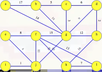
and ends as

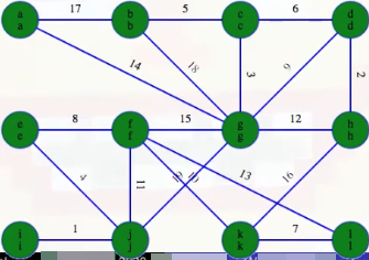
after a top-level DFS (the top character of each node represents the node itself, and the bottom character represents the component representative from the top-level DFS). A total of $|V|$ top-level depth-first searches are conducted in the first phase. But no matter what phase we're in, there are fewer edges than vertices so it's always going to be a quick search (recall that if a tree has x nodes, then it must have x - 1 edges, and a subtree is itself a tree).

Each vertex in any forest tree will get marked with the first vertex that was searched in its component; that is, as stated above, the top character of each node represents the node itself, and the bottom character represents the component representative from the top-level DFS (e.g., if we start a top-level DFS on node x and somehow get to nodes y and z during this search, then bottom character in nodes x, y, and z will be x).

We can then use that vertex to store the minimum weight edge out of the component, maybe initializing it with infinity. To actually find the minimum weight edges leaving each tree, go through every edge e = (u, v) in G:

Boruvka(G = (V, E)) {
    T = Ø
    while(|T| < |V| - 1) {
        initialize each vertex to an unknown component
        discover each T_i by running DFS on (V, T)
            each v discovered by the top level DFS indicates a new component
            initialize each with an infinite weight edge
        for(e = (u, v) in E)
            if(u's component != v's component)
                update u's component's minimum weight edge if needed
                update v's component's minimum weight edge if needed
        add those edges to T
    }
    return T
}

If the edge's vertices are in different components, then check each edge in each component to see if edge e is a new minimum edge. It's possible for the edge to be the minimum out of neither, either, or both trees.

Algorithm

After we've finished looking at all of the edges, each component stores an edge that should be added to the MST. So add it (just remember: an edge can only be added once even if it's the minimum weight edge out of two different components; after that, if we still have more than one tree in our forest, then we reset the components and run another phase, and that's it):

Boruvka(G = (V, E)) {
    T = Ø
    while(|T| < |V| - 1) {
        initialize each vertex to an unknown component
        discover each T_i by running DFS on (V, T)
            each v discovered by the top level DFS indicates a new component
            initialize each with an infinite weight edge
        for(e = (u, v) in E)
            if(u's component != v's component)
                update u's component's minimum weight edge if needed
                update v's component's minimum weight edge if needed
        for each component T_i
            add T_i's minimum weight edge to T
    }
    return T
}

What does this mean in the context of the sample graph we've been considering? Recall that the first part of the first phase involved discovering components (lines 4-7 above), and it wasn't very exciting for the first phase — we started with the figure on the left and ended with the figure on the right after all the top-level depth-first searches concluded:

Lines 8-11 let us identify the minimum weight edge associated with each component (identified by heavy blue edges in the figure on the left), and we then need to add these edges to the MST per lines 12-13 (MST edges are highlighted in red):

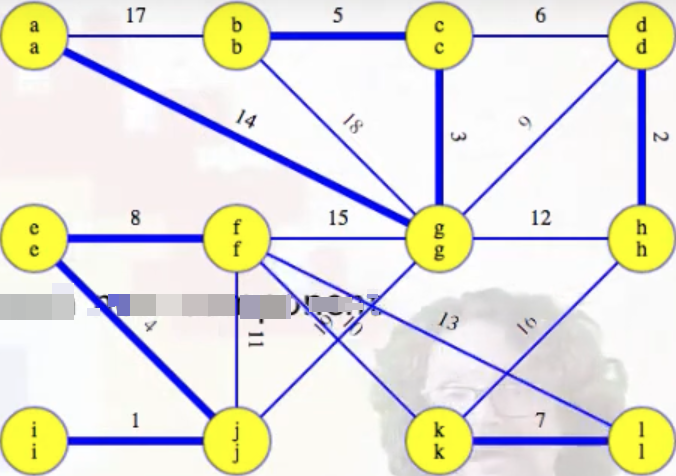
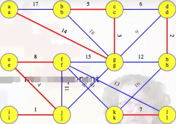
Example (second phase)

What happens next in our example graph? We're ready for the second phase. As indicated by the pseudocode, each vertex is first initialized to an unknown component (line 4):

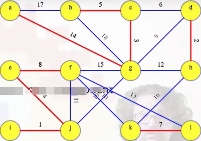
But now our top-level depth-first searches will yield something interesting (unlike in the first phase). The first phase concluded by ultimately adding eight edges to our MST, highlighted in red above (edges are grouped in the list based on now being part of the same T_i):

T = [
  (a, g), (g, c), (c, b), # T_1
  (d, h),                 # T_2
  (e, f), (e, j), (i, j), # T_3
  (k, l)                  # T_4
]

What will the second phase yield? Using the image above that shows our current graph state as well the list of edges in T thus far, we can actually deduce this somewhat easily for ourselves.

Assuming we start all top-level depth-first searches in alphabetical order (for the sake of consistency), we can note which vertex is discovered first for each subtree:

T = [
  (a, g), (g, c), (c, b), # T_1: a
  (d, h),                 # T_2: d
  (e, f), (e, j), (i, j), # T_3: e
  (k, l)                  # T_4: k
]

What are the minimum weight edges coming out of each of the components above (i.e., edges that do not connect vertices within the same component)? After iterating through all edges and iteratively updating the minimium weight edge reference for each component, we have the following:

# <vertices in component>: <minimum-edge-weight-out-of-component> # <min-weight-edge>
{
  'abcg':   6   # (c-d)
  'dh':     6   # (d-c)
  'efij':   10  # (f-k)
  'kl':     10  # (k-f)
}

The simple observations above show us that the four edges (c, d), (d, c), (f, k), and (k, f) will be added to the MST; of course, since (c, d) and (d, c) refer to the same edge, and (f, k) and (k, f) also refer to the same edge, we really end up only adding two edges to the MST.

And this is exactly what happens.

The top-level depth-first searches for the second phase give us the following:

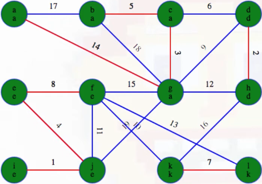
Note that this is exactly what we suspected:

T = [
  (a, g), (g, c), (c, b), # T_1
  (d, h),                 # T_2
  (e, f), (e, j), (i, j), # T_3
  (k, l)                  # T_4
]

It may help if we highlight and magnify each component:

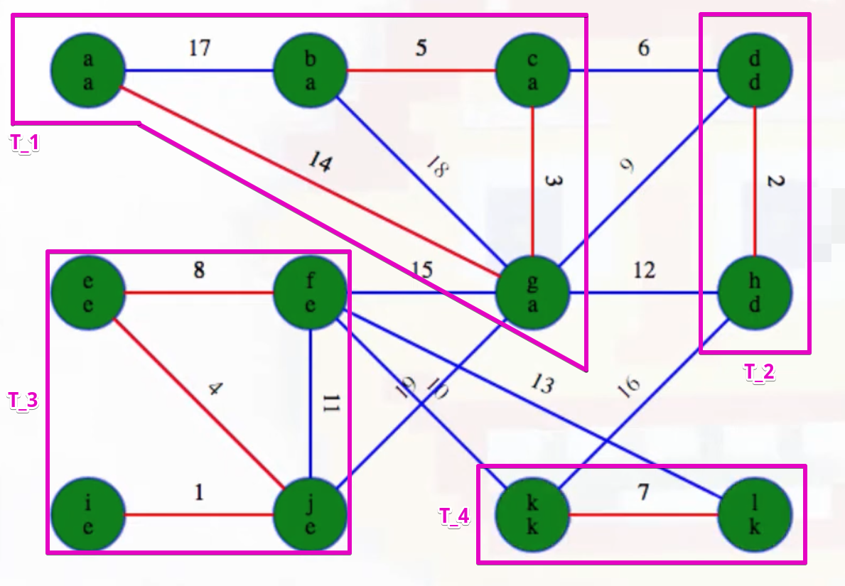
Now highlight the minimum weight edge leaving each component (highlighted in heavy blue):

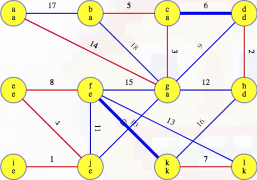
Add these edges to the MST:

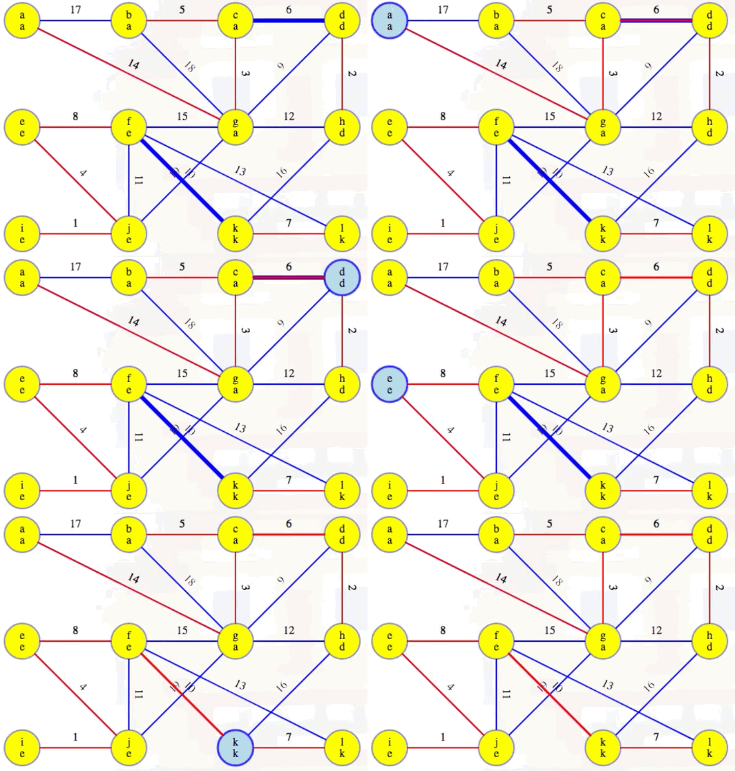
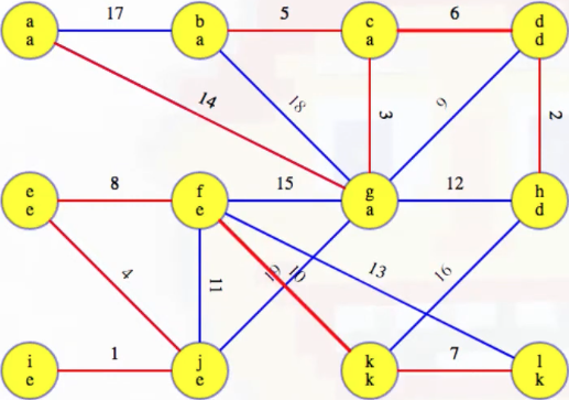
Our MST at the end of the second phase is as follows, with edges (c, d) and (f, k) now included, as expected:

Example (third phase)

The third phase should now be a bit easier to understand. Remember, each vertex is first initialized to an unknown component (line 4):

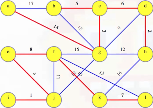
Again, assuming we start all top-level depth-first searches in alphabetical order (for the sake of consistency), we can note which vertex is discovered first for each subtree:

T = [
  (a, g), (g, c), (c, b), (c, d), (d, h) # T_1: a
  (e, f), (e, j), (i, j), (f, k), (k, l) # T_2: e
]

We can this is the case just by introducing a black line to separate the subtrees:

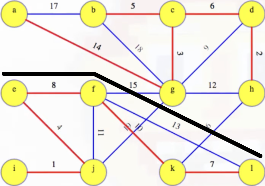
When we find the components via depth-first searches, we can tell all vertices above the black line in the image will have label a, and all vertices below the black line will have label e. And this is exactly what happens:

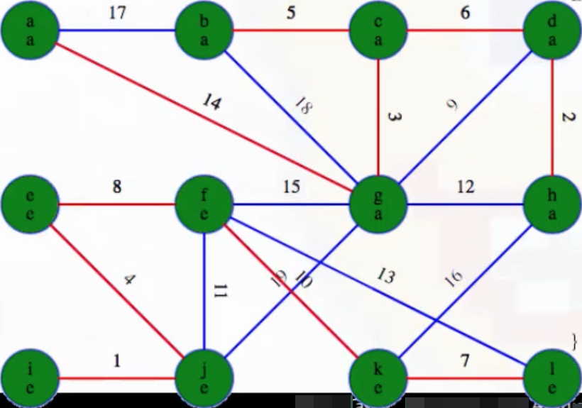
What are the minimum weight edges coming out of the components we've identified? The image with the black line separating the subtrees makes this easier to identify. There are only three edge possibilities:

• (f, g) with weight 15
• (j, g) with weight 19
• (k, h) with weight 16.

Clearly edge (f, g) is the optimal choice here, and we can see this from both component:

# <vertices in component>: <minimum-edge-weight-out-of-component> # <min-weight-edge>
{
  'abcdgh':   6   # (g-f)
  'efijkl':   6   # (f-g)
}

We can this highlighted in our image (heavy blue), as expected:

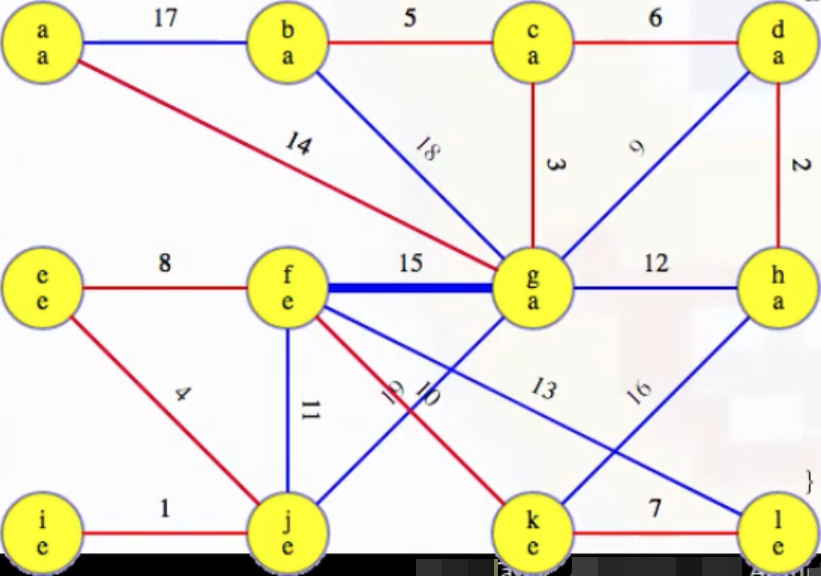
And then we can see this edge added to the MST:

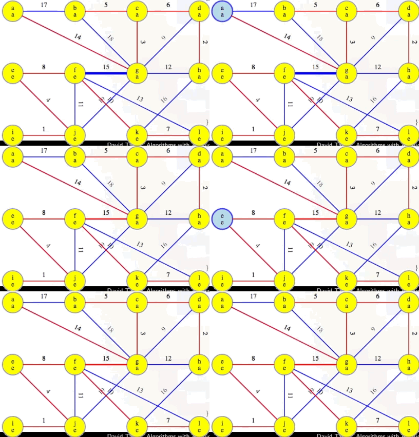
Is there a fourth phase? No. Why? At this point, the MST we've been building, T, now has V - 1 edges (i.e., |T| == |V| - 1), which means our while loop condition |T| < |V| - 1 is no longer met, preventing us from pursuing a fourth phase, as desired and expected.

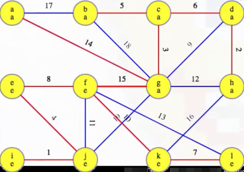
T now holds the final MST for our example graph:

Analysis

Let's first highlight the significant steps in our algorithm from a runtime standpoint:

Boruvka(G = (V, E)) {
    T = Ø
    while(|T| < |V| - 1) {
        initialize each vertex to an unknown component                        # Θ(|V|)
        discover each T_i by running DFS on (V, T)                            # Θ(|V|)
            each v discovered by the top level DFS indicates a new component
            initialize each with an infinite weight edge
        for(e = (u, v) in E)                                                  # Θ(|E|)
            if(u's component != v's component)
                update u's component's minimum weight edge if needed
                update v's component's minimum weight edge if needed
        for each component T_i                                                # O(|V|)
            add T_i's minimum weight edge to T
    }
    return T
}

Finding components takes time linear in the number of vertices. Finding the minimum edge for each component takes time linear in the number of edges. And adding edges to the MST takes time linear in the number of components, which is bounded by the number of vertices.

So each phase takes time linear in the size of the graph. Each phase has no more than half as many components as the previous phase. So we get at most \lg |V| phases for worst-case order $|E|\lg |V|$ runtime: $O(|E|\lg|V|)$.

But unlike Kruskal's algorithm, where sorting the edges at the beginning really does usually take $|E|\lg|V|$ time, we might end up with a lot fewer phases in Boruvka's algorithm.

Optimizations

If we're willing to add a bit of complexity to our code, then there are some optimizations we can make, specifically by "shrinking our graph" between phases: remove any edge from consideration that doesn't leave a component, and if we have multiple edges between two different trees in our forest, throw them all away except the cheapest. Then we can shrink each forest tree down to a single vertex for our next phase. We can see how that could help us in a complete graph. Even if we have as many phases as possible, if we halve the number of vertices each round, then that would basically quarter the number of edges. Each round should take less than half as long as the round before it for linear total runtime.

But we can also get linear runtime for less dense graphs from Prim's algorithm. However, Boruvka's algorithm gives a worst-case linear runtime for other types of graphs, including planar graphs and some other sparse graph types.

To recap:

• $O(|E|\lg|V|)$ worst-case runtime but frequently faster (unlike Kruskal's)
• To optimize, contract $G$ along new edges from $T$ each phase:
  • From edge list, discard each edge between two vertices in one component.
  • Discard all but the edge of minimum weight between two components.
  • Treat each component as a single vertex for the next iteration.
  • Linear worst-case time on planar graphs, other graph families too.
• For dense graphs, Prim's algorithm will be linear for $|E| = \Omega(|V|\lg|V|)$.

Prim's algorithm

Idea

Like our other algorithms, we start with a forest of single-vertex trees for every vertex in the graph. But unlike Kruskal and Boruvka, there's one "special" (but arbitary) vertex from that forest, say vertex a. a's tree is special for this algorithm. We will repeatedly find the minimum edge weight leaving it and add it to our forest. It doesn't look so much like a bunch of different trees being merged together in the forest; instead, it looks more like a single tree, growing to take over the rest of the graph, assimilating it like the Borg would. It still fits our generic algorithm mold, but all of the trees in the forest, except one, are singleton vertices.

Let's recap what we have so far:

• Start with a "special" (but arbitrary) vertex a. Call its forest tree T_a.
• Add minimum weight edge between T_a and the rest of the graph.
• Keep doing that until T_a covers the graph.

Outline

What we described above is Prim's general outline:

Prim(G = (V, E)) {
    tell arbitrary vertex a that it is "special"
    while (not done yet) {
        add minimum weight edge between T_a and rest of the graph
    }
    return tree
}

Step by step, we'll replace the outline with the actual algorithm.

We want to efficiently track the minimum weight edge from the special tree, T_a. That edge must lead to one of the vertices not yet in the tree. For each vertex not in the tree, store its minimum weight edge from the special tree as a potential minimum spanning tree. We put those edges into a priority queue:

Prim(G = (V, E)) {
    tell arbitrary vertex a that it is "special"
    create a min priority queue Q to "v not in T_a" with lightest edge T_a to v
    while (Q not empty) {
        add minimum weight edge between T_a and rest of the graph
        update Q to hold updated minimum weights from new, bigger T_a
    }
    return tree
}

The key/priority for each vertex, v, in the queue, Q, is the weight of the edge from our special tree, T_a, to reach that vertex v. Adding initialization to our outline, every vertex gets initiailized with an infinite key:

Prim(G = (V, E)) {
    for each v in V
        v.heapKey = inf, v.MSTEdge = NIL
    tell arbitrary vertex a that it is "special"
    create a min priority queue Q to "v not in T_a" with lightest edge T_a to v
    while (Q not empty) {
        add minimum weight edge between T_a and rest of the graph
        update Q to hold updated minimum weights from new, bigger T_a
    }
    return tree
}

Our special vertex, however, gets a priority or heap key of 0:

Prim(G = (V, E)) {
    for each v in V
        v.heapKey = inf, v.MSTEdge = NIL
    for arbitrary "special" vertex a, a.heapKey = 0
    create a min priority queue Q with all vertices
    while (Q not empty) {
        add minimum weight edge between T_a and rest of the graph
        update Q to hold updated minimum weights from new, bigger T_a
    }
    return tree
}

That will be the first vertex out of the queue.

Running example (first vertex)

Prim(G = (V, E)) {
    for each v in V
        v.heapKey = inf, v.MSTEdge = NIL
    for arbitrary "special" vertex a, a.heapKey = 0
    create a min priority queue Q with all vertices
    while (Q not empty) {
        u = Q.ExtractMin
        mark u as not in Q
        for(each edge e = (u, v))
            if(v in Q)
                if(e.weight < v.heapKey)
                    v.MSTEdge = e
                    Q.DecreaseKey(v, e.weight)
    }
    return tree
}

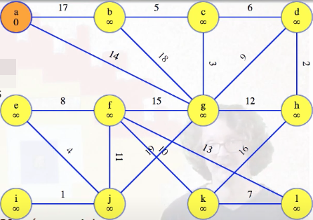
In the running example, when a vertex is removed from the queue, it will be marked orange. The graph's starting state, after initialization and once the special vertex is popped from the heap (i.e., dequeued from the priority queue), is basically the following:

We have to consider that current orange vertex's edges to the other vertices still in the queue. For the first vertex, of course any edge is better than nothing, so we'll replace the dummy "infinity edges" with the edges from a, and update the queue:

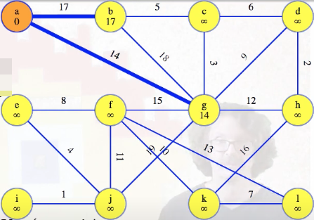
The heavy blue edges in the image above, stored with the vertices still in the queue, should be thought of as potential MST edges. They haven't been ruled out yet. Once we're done with all edges from our special vertex, a in this case, we finish it and mark it blue:

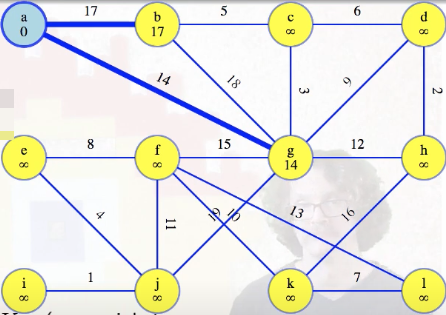
Right now each vertex in the queue holds a potential MST edge, its minimum weight edge reaching it from the special tree, which is just vertex a in this case.

Running example (second vertex)

Whenever that's true, we can justify removing the vertex with the lightest edge from the queue, and including its edge in the MST:

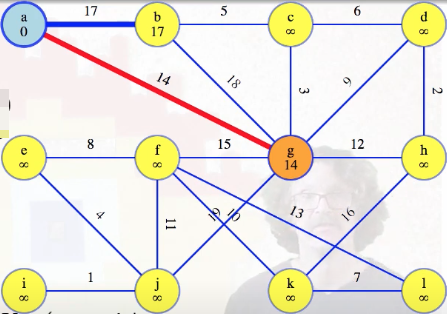
The new red edge above is the lightest edge crossing the cut between our special tree and the rest of the graph. By the cut crossing theorem, this edge must be in the MST. That's the way it works with every vertex after the first one.

Algorithm

Before removing a vertex from the queue, the queue holds all vertices not yet in the tree, and each vertex holds its lightest weight edge to a's tree. One edge for each vertex, except the first, gives us |V| - 1 edges total:

Prim(G = (V, E)) {
    for each v in V
        v.heapKey = inf, v.MSTEdge = NIL
    for arbitrary "special" vertex a, a.heapKey = 0
    create a min priority queue Q with all vertices
    while (Q not empty) {
        u = Q.ExtractMin
        mark u as not in Q
        for(each edge e = (u, v))
            if(v in Q)
                if(e.weight < v.heapKey)
                    v.MSTEdge = e
                    Q.DecreaseKey(v, e.weight)
    }
    return {v.MSTEdge | v in V, v != a}
}

Before the second vertex, g, the only edges in the queue are direct edges to a. Those are definitely the minimum weight edges from each queue vertex back to a's single-vertex tree. g's edge of weight 14 grows a's tree, so we should update the lightest edges to all of the vertices still in the queue. The lightest edge might still come from a, but now it could also come from g. We consider all edges out of the new vertex. If the edge leads to something already in the tree, then ignore it because we've already looked at those edges from the other side (that's only the edge to a here). But for the edge from g to b, we could already reach vertex b for cost 17 — that's better than 18. So we discard the 18 edge (faded blue):

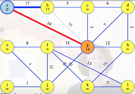
We won't ever use it, and we won't ever have to change our mind about it. We can see that it's the maximum weight edge on a cycle; thus, by the cycle theorem, the weight 18 edge from g to b definitely won't be in our final MST.

All of the other vertices that g has an edge to previously stored infinity values so they all get new weights for their edge from g, and the priority queue gets updated after each change:

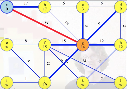
Eventually, we finish with all edges from g:

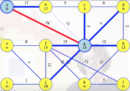
By checking all of the edges from that vertex, we've updated the edges from our tree to the vertices still in the queue. So each vertex still holds its lightest weight edge to our growing tree, and, collectively, they hold the lightest edge from that tree.

Running example (vertices 3-5)

Let's generalize those arguments. When we're ready to take another vertex from the queue, such as vertex c,

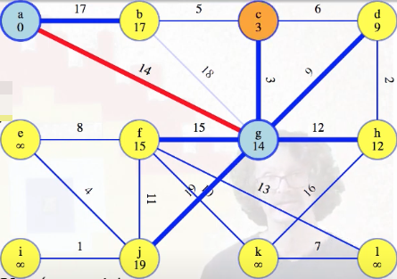
we assimilate it and the edge reaching it into our growing tree, which will always be a subtree of the MST:

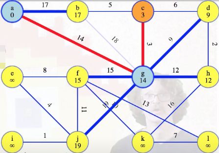
When we are preparing to remove a vertex u from the queue, such as vertex c above, we look at all edges (u, v) incident on vertex u and update the minimum weight edge associated with each vertex v. For example, when we consider vertex c above, the first thing we do is look at edge (c, b), where we see right now vertex b has a recorded minimum weight edge of 17 to our special tree. But vertex c is now part of our special tree, which means vertex b could be connected to our tree now by edge (c, b) instead of (b, a); that is, the minimum weight edge associated with vertex b should now be updated to be 5 instead of 17 (this also means we should remove edge (b, a) from future consideration because now it would the maximum weight edge on a cycle):

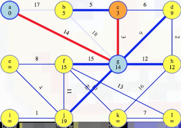
We then also look at edge (c, d), and see that d should now hold a minimum edge weight of 6, instead of its previously held minimum edge weight of 9 (this results in removing edge (g, d) from consideration because then its edge would be a maximum weight edge on a cycle):

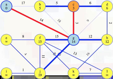
Now that vertex c has been fully processed, we can remove it from the queue and mark it as finished:

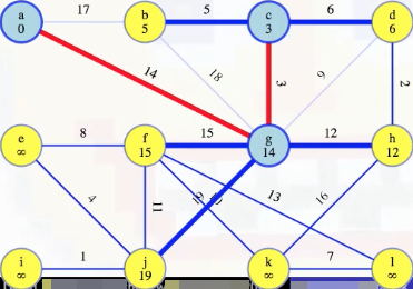
Now we look at vertex b, which is an easier consideration, because there's only one edge to consider for its minimum weight edge to our special tree (due to previous edge consideration eliminations):

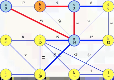
Now we need to update all outgoing edges from b, but all of these edges have already been eliminated from consideration (i.e., (b, a) and (b, g)) or are already in the MST (i.e., (b, c)). So we can remove it from the queue and mark it as finished:

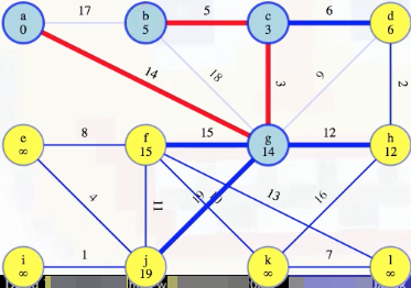
Now we prepare to remove vertex d from the queue:

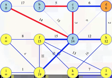
The minimum edge weight from vertex d to our special tree is (d, c) with weight 6, so we add it to our special tree:

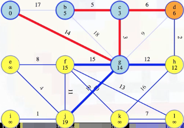
Now we need to update the minimum weight edges associated with each vertex v for vertices incident on (d, v). We just added the edge (d, c) to our MST so vertex c's associated minimum weight edge doesn't need to be updated. And we've already eliminated edge (d, g) from consideration so vertex g's associated minimum weight doesn't need to be updated either. The only other possibility is edge (d, h). The minimum edge weight to our MST currently associated with h is 12, but since d is now part of our MST, the edge (d, h) of weight 2 now means vertex h has a minimum edge weight of 2 from our special tree (this means we should also remove edge (h, g) from consideration now since it would be the maximum edge weight on a cycle):

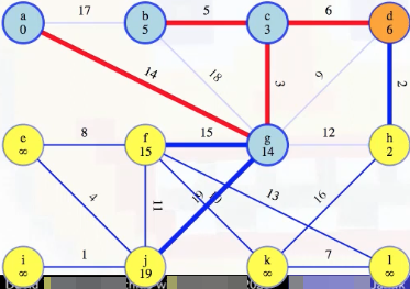
Let's describe in a more formal/general way what all we just did to add vertices c, b, and d to our MST. At the beginning of this section, we mentioned that when we're ready to take another vertex from the queue, such as vertex c, we assimilate it and the edge reaching it into our growing tree, which will always be a subtree of the MST. Because the queue held the lightest weight edges from our tree to the vertices in the queue, the lightest weight edge in the queue is definitely in the MST. So when we add it to our growing tree, we maintain that it is a subtree of the minimum spanning tree.

The lightest edge from the updated tree to any vertex still in the queue either comes from the new vertex or from one of the vertices in the tree before it grew. We had already computed and stored those in the queue. Those are the only possibilities. We look at each edge incident on the new vertex.

Running example (sixth vertex)

Let's consider now what happens when we get to vertex h:

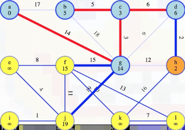
As we did above, we can ignore any edge from a vertex already in a's special tree. It is either the edge we just added to the MST, (h, d), or it's an edge we previously discarded. At all times, every edge is one of the following:

• known to be in the MST
• discarded
• stored in the queue
• not yet seen

Edges are seen first from whichever vertex is included into a's tree first. So edges to vertices already in the MST have been seen. For those edges, both vertices are already out of the queue. So we've already determined if those edges are in the MST or not. Ignore them.

If the edge leads to a vertex still in the queue, such as (h, k)

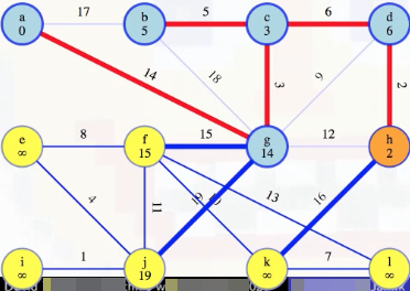
then check to see if it's a better way to connect that vertex to the tree. We compare the previous best weight to reach it against the edge weight from our current vertex; keep whichever is smaller and discard the other. In this case, the previous minimum edge weight from k to a's special tree was infinity, but now that h is included in a's special tree, we see that the edge (h, k) with edge weight 16 means that now the minimum edge weight from k to our special tree is 16 instead of infinity:

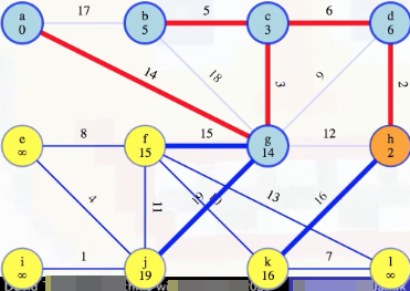
Above, we didn't really "discard the other" because we previously couldn't even reach our MST from k.

Running example (seventh vertex)

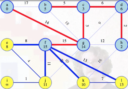
But what about when we take f our queue?

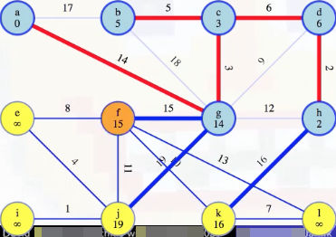
First things first, we add the minimum weight edge to our MST:

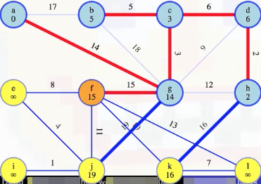
Then we start the process of updating the minimum edge weights associated with each vertex, updating e's to be 8 (it previously wasn't reachable), j's to be 11 (it was previously 19), but what about k? We can see there's a weight 10 edge from f to k:

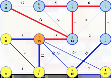
We compare this with the weight 16 edge that was previously the best way to reach k from h, and we'll throw one of these edges away. Because f and h are now both in the growing tree, they're connected by edges in that tree, specifically edges 15, 3, 6, 2 (i.e., (f, g), (g, c), (c, d), (d, h)), which we know are all part of the MST. Hence, taking that path, f-g-c-d-h, plus the (f, k) and (h, k) edges, gives a cycle: f-k-h-d-c-g-f. The heaviest edge on that cycle is not in the MST by the cycle theorem. The heaviest edge clearly can't be any of the edges on the MST tree path from f to h because we've used the cut crossing theorem to show those edges are in the MST. So it has to be one of the last two edges, (f, k) or (h, k):

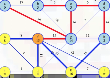
This justifies discarding the heavier of those two edges forever:

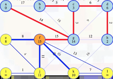
It's the heaviest in a cycle. Now we just need to update the minimum weight edge associated with l from f (previously unreachable):

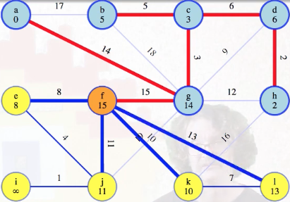
Then vertex f can be marked as completed:

Running example (remaining graph)

Let's recap the process we've described before completing processing the rest of the graph:

• Just before removal from $Q$, $v\in Q$ holds its minimum weight edge to $T_a$.
• The minimum of those edges is the minimum edge leaving $T_a$. It is in the minimum spanning tree by the cut crossing theorem.
• After adding some $u$ and its edge to $T_a$, consider each edge $u$, $(u, v)$.
• If $v$ is already in $T_a$, then ignore $(u, v)$ as it has already been classified. There are only four kinds of edges:
  • Known in MST
  • Discarded
  • Stored in $Q$
  • Not yet seen
• If $v$ is still in $Q$, then compare its edge in $Q$ against $(u, v)$. The larger is the heaviest in a cycle and can safely be discarded by the cycle theorem.

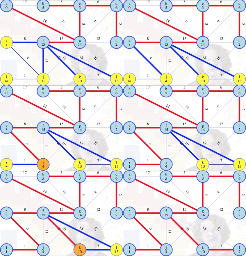
Following the process above, the remainder of the graph can be processed as follows:

Comparison to Dijkstra's

Recall our pseudocode for Prim's algorithm:

Prim(G = (V, E)) {
    for each v in V
        v.heapKey = inf, v.MSTEdge = NIL
    for arbitrary "special" vertex a, a.heapKey = 0
    create a min priority queue Q with all vertices
    while (Q not empty) {
        u = Q.ExtractMin
        mark u as not in Q
        for(each edge e = (u, v))
            if(v in Q)
                if(e.weight < v.heapKey)
                    v.MSTEdge = e
                    Q.DecreaseKey(v, e.weight)
    }
    return {v.MSTEdge | v in V, v != a}
}

This looks a lot like what's needed for Dijkstra's single-source shortest path algorithm. But Dijkstra's algorithm really has an actual special vertex, the source.

For Prim's algorithm, we don't really even need to mark a special vertex. We could have left the special vertex's weight at infinity (remove line 4 above). Whatever arbitrary infinity-weight vertex the priority queue spits out first would be our "special" vertex (i.e., the vertex we start with in Prim's algorithm is truly arbitrary):

Prim(G = (V, E)) {
    for each v in V
        v.heapKey = inf, v.MSTEdge = NIL
    create a min priority queue Q with all vertices
    while (Q not empty) {
        u = Q.ExtractMin
        mark u as not in Q
        for(each edge e = (u, v))
            if(v in Q)
                if(e.weight < v.heapKey)
                    v.MSTEdge = e
                    Q.DecreaseKey(v, e.weight)
    }
    return {v.MSTEdge | v in V, v.MSTEdge != NIL }
}

Analysis

Since the code for Prim's algorithm is quite similar to the code needed for Dijkstra's algorithm, it isn't surprising that the analysis is similar.

The algorithm takes linear time, excluding the priority queue operations. |V| extractions empty the queue. And, up to once for each edge, we might decrease the key of something in the queue. If we use a binary heap as a queue, then that will give us $O(|E|\lg|V|)$ time. If, however, we use a Fibonacci heap, which takes constant average time to decrease a key and average logarithmic time to extract the minimum, then it takes $O(|E| + |V|\lg |V|)$ time. If the graph has at least $|V|\lg|V|$ edges, then that's linear run time.

In summary:

• Initialization: $O(|V|)$
• Cycle through each edge, excluding priority queue operations: $O(|E|)$
• $|V|$ ExtractMin remove min operations from priority queue
• $O(|E|)$ DecreaseKey operations
• $\Theta(|E|\lg|V|)$ worst-case runtime with binary heap priority queue
• $\Theta(|E| + |V|\lg|V|)$ worst-case runtime with Fibonaccni heap priority queue, and linear for graphs with $|E| = \Omega(|V|\lg|V|)$.

Interactive examples

Coming soon.

---