Graphs: basics (with attitude)

This post explores the basics of graphs. Specifically, we start by considering what graphs actually are (i.e., as a concept). Then we discuss a variety of ways to represent graphs in code. Then we move on to the two most fundamental graph traversal techniques: breadth-first search (BFS) and depth-first search (DFS).

Attribution

The notes below come from the Algorithms with Attitude YouTube channel, specifically the Graphs: Basics playlist comprised of the following videos: Introduction to Graphs, Graphs: Representation, Graphs: Breadth First Search (BFS) with Example, and Graphs: Depth First Search (DFS) with Example.

There are several sections in this post, accessible in the table of contents on the right, but most of the sections have been listed below for ease of reference and navigation.

• Introduction to graphs
  • Basic definition
  • Undirected graph (Facebook)
  • Directed graph (webpages)
  • Edge interpretation
  • Edge direction
  • Weighted graphs: flow problems
  • Shortest path problems
  • Clustering problems
  • Examples
  • Terminology recap
• Representations of graphs
  • Graph vs. representation
  • Adjacency matrix
  • Sentinel weights
  • Undirected graph matrices
  • Adjacency list
  • List variants
  • Undirected adjacency lists
  • Outgoing and incoming lists
  • Transformations between lists
  • Transforming adjacency list to adjacency matrix
  • Transforming adjacency matrix to adjacency list
  • Graph transpose
  • Representation comparison (space)
  • Representation comparison (time)
• Breadth first search (BFS)
  • Basic idea
  • Simple imlpementation
  • Full implementation
  • Queue observation
  • Reconstructing shortest paths
    • Recursive pseudocode
    • Iterative pseudocode
    • Python implementations
  • Cormen colors
  • Analysis
  • Handwavey correctness outline
• Depth first search (DFS)
  • Basic idea
  • Simple implementation
  • Full implementation
  • Vertex vs. graph DFS
  • Example
  • Parenthesis notation
  • Cormen vertex colors
  • Edge classifications
  • Analysis
  • Concern for potential stack overflow
  • Iterative DFS with a stack

Introduction to graphs

Graphs are one of the most important, versatile, and widely used data structures out there. Right now we'll mostly talk about how to use graphs to model a few domains. But let's start by defining the absolute basics.

Basic definition

As noted on WikiPedia, a graph is a set of vertices/nodes and a set of edges between vertices; that is, mathematically, graph is a pair $G = (V, E)$, where $V$ is a set whose elements are called vertices, and $E$ is a set of pairs of vertices, whose elements are called edges.

In brief:

• Graph: A set of vertices and a set of edges.
• Vertex (or node): Represents some entity.
• Edge: Connects two vertices; that is, an edge represents a relation between the two vertices.

Undirected graph (Facebook)

Suppose we have a "graph for Facebook", where each vertex represents a person, and an edge between people means those people are friends. Edges represent some relationship between the vertices they connect (i.e., Facebook friends in this example). For graphs, we say such vertices are adjacent and that an edge is incident on its vertices.

Just for scale, Facebook is a pretty big graph with over a billion vertices and hundreds of billions of edges. So what does it mean if we have our privacy settings set so that only our friends can see our posts? Those are our vertex neighbors in the graph. But if we change our settings so that friends of friends can see our posts, then that adds all vertices on a path of length 2 away from ourself. The number of edges connected to a vertex is its degree. If we want to link out further, then how many people will we reach if we allow three or four edges? How about if we just allow anybody with any path from ourself? That would be all vertices reachable from ourself in the graph.

Directed graph (webpages)

For a bigger graph, think of the graph of webpages. Each webpage is a vertex with an edge to another webpage if it has a link to that page. Notice that there's a fundamental difference between this graph and the Facebook graph. For Facebook, the "friendship" relation is symmetric; that is, person A is friends with person B if and only if person B is friends with person A. When all relations have to be symmetric in a graph, then such a graph is said to be undirected. Webpages aren't like that. Webpage A can link to webpage B, but webpage B doesn't have to link back to webpage A. This is an example of a directed graph or digraph, and we usually place an arrow on the edge to indicate the direction of the edge.

Of course, webpages can link to each other, so we can have an edge in each direction between two vertices. That makes a cycle of length 2 (i.e., a path that ends up where it started). For a cycle, it really doesn't matter which vertex we consider to be the "start" vertex. If a cycle contains no smaller cycles, then it's called a simple cycle, and if a path has no repeated vertices, then the path is said to be a simple path. Directed graphs with no cycles at all are called directed acyclic graphs (DAGs). Cycles in undirected graphs are similar, but to be clear, if an edge from A to B in an undirected graph exists, then we don't consider this edge itself to be a cycle just because we can get back from B to A on the same edge; that is, we have something like the following:

C to A to B to A to C -> not a cycle
C to A to B to D to C -> cycle

Edge interpretation

For webpages, it makes sense to think of edges going from the page with the link to the linked page. What do links tell us about a page? What does it mean if a page has a high in-degree? Such a page is probably an authoritative or expert page/reference on something. Lots of other pages are linking to it for some reason.

For example, if 1000 different webpages are all talking about butterflies, and they all have a link to one page, then that page probably has something to do with butterflies even if it doesn't have the word "butterfly" anywhere on the page. That's one of the ways that Google can figure out what pages to highly rank for different search terms even if the term doesn't appear in the page.

On the other hand, think about pages with a high out-degree (e.g., WikiPedia pages). Pages with a high out-degree are probably a directory or collection of some kind.

Edge direction

Depending on what we're modeling, sometimes edge direction won't be so obvious. In Twitter, you might want to think about who you follow and model an account with the edges to those the account follows. Or, maybe instead we want to think about the flow of information.

• Link to those followed? (Follow the interest.)
• Link to followers? (Follow the information.)

When we model the graph, we need to decide what edge direction we want to use. Either way is fine, but we need to aim to be consistent.

Weighted graphs: flow problems

The examples discussed so far seem a bit similar, but we can also use graphs to model more physical, real-world things too. The physical communication channels of the internet itself can be modeled by a graph (i.e., submarine cables). In that case, we may want to model some extra information for each edge like the "capacity" for that edge (e.g., how much data it can carry). We can store that data with the edge, and we call the graph as a whole a weighted graph. If we want to figure out where to lay our next cable for more robust connectivity or maximize data flow between two locations, then that's a connectivity or flow problem. In weighted graphs, what the weight means is completely dependent on what we're modeling.

Shortest path problems

If we're modeling a flight, then an edge weight might represent the cost of a flight from an origin to a destination or possibly the duration for that flight. If we want to minimize the cost or the duration (or possibly some combination of both), then we have a path minimization problem. The edge weights can really stand for whatever thing we're trying to optimize.

Clustering problems

If we have a seating chart (e.g., for a wedding), then an edge weight might represent how much our aunt despises the groom's best man. We're trying to seat tables in order to minimize how unhappy our guests are. That's a clustering problem.

Examples

Graphs are so versatile that it's hard to say what a "typical" graph problem looks like. They can be used to map shortest distances, find cheap flights, minimize wire lengths, plan bus routes, optimize cable placement, choose warehouse locations, decrease gasoline usage, schedule classes, recommend friends, plan parties, solve Rubik's Cube, etc., etc.

Unsurprisingly, depending on what we choose to model, there will be some differences in what we want to allow:

• directed or undirected?
• weighted?

The above are probably the biggest differences, but there can also be more minor questions like whether or not a vertex can have an edge to itself (called a loop). For any particular problem we're modeling, loops may or may not make sense. On the other hand, graphs only allow one edge between two nodes (undirected) or one in each direction (directed).

Multigraphs allow parallel or multi-edges. Hypergraphs allow hyperedges, each between an arbitrary set of vertices.

Terminology recap

• adjacenct vertices share an edge
• an edge is incident on its vertices
• a vertex's neighbors are the vertices adjacenct to it
• vertices in a sequence connected by edges form a path
• the number of edges in a path is the path's length
• the edge count for a vertex is its degree
• if a path goes from one vertex to another, then the latter is reachable from the first
• all edges in undirected graphs go both ways
• edges in directed graphs (digraphs) go one way
• a cycle is a path back to its start vertex
• a simple cycle contains no other cycles
• a simple path contains no cycles
• an acyclic graph contains no cycles
• a DAG is a directed acyclic graph
• the number of directed edges pointing to a vertex is its in-degree
• the number of directed edges pointing from a vertex is its out-degree
• in a weighted graph, each edge has an associated weight
• connectivity: how connected is the graph?
• flow: how much capacity is there in a network?
• path minimization: minimize sum of edge weights on a path
• clustering: partition vertices to optimize some function of the weights between them

Representations of graphs

Graph vs. representation

Suppose we have a sort of abstract graph with vertices and edges (each of which represents some kind of information and relation):

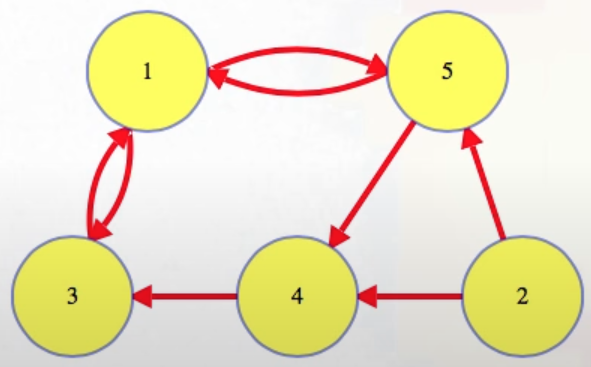
The graph representation we choose is just some implementation which captures that abstract graph information. But we can come up with different implementations to capture the same graph; that is, the exact same graph may be represented in very different ways. The two most common ways to represent a graph are the adjacency matrix and adjacency list. The names of these representations demonstrate how they choose to convey the structure of the graph, namely by detailing adjacencies in matrix or list form (recall that two vertices are said to be adjacent if they share an edge).

Adjacency matrix

The normal way to represent a graph with an adjacency matrix is to use a 2D matrix. We assume that vertices are numbered (if a graph has n vertices, then the vertices are usually labeled 0 to n - 1 when working with code, but it's commonplace to see the vertices labeled 1 to n when discussed in a more academic context). If an edge in the graph exists from i to j, then the adjacency matrix will hold some information about this edge in row i and column j. What's actually stored in the adjacency matrix? In the simplest case, only a single bit is stored, namely a true (the edge exists) or false (the edge does not exist) boolean. The true and false booleans are also sometimes stored as the values 1 and 0, respectively.

For example, the previously pictured graph can be represented as follows:

$$\begin{array}{c|ccccc} {} & 1 & 2 & 3 & 4 & 5\\\hline 1 & \text{F} & \text{F} & \color{red}{\text{T}} & \text{F} & \color{red}{\text{T}}\\ 2 & \text{F} & \text{F} & \text{F} & \color{red}{\text{T}} & \color{red}{\text{T}}\\ 3 & \color{red}{\text{T}} & \text{F} & \text{F} & \text{F} & \text{F}\\ 4 & \text{F} & \text{F} & \color{red}{\text{T}} & \text{F} & \text{F}\\ 5 & \color{red}{\text{T}} & \text{F} & \text{F} & \color{red}{\text{T}} & \text{F} \end{array}$$

In the most complex case, we could store an edge object instead of a boolean that contains a variety of key-value pairs (e.g., weight, name, likes, etc. ... whatever we need for the problem we're modeling). A common case between the two extremes of just a boolean or a full object is when we just need an edge weight:

In such cases, instead of storing a true/false value, we store the edge weight:

$$\begin{array}{c|ccccc} {} & 1 & 2 & 3 & 4 & 5\\\hline 1 & {} & {} & \color{red}{146} & {} & \color{red}{6046}\\ 2 & {} & {} & {} & \color{red}{180} & \color{red}{155}\\ 3 & \color{red}{18063} & {} & {} & {} & {}\\ 4 & {} & {} & \color{red}{6001} & {} & {}\\ 5 & \color{red}{255} & {} & {} & \color{red}{42} & {} \end{array}$$

Sentinel weights

But what do we store if there's no edge? Some programming languages might allow us to store nil or a null reference, but even then, each time we need an edge weight, we first need to see if the edge exists, and then use it. This can slow our code down a bit and also makes it clunky in some situations. Instead, depending on what the weights represent, it's common to store a dummy weight or "sentinel value" for missing edges. For example, if weights represent something we're trying to minimize (like a cost), then we store a huge value by default (like infinity):

$$\begin{array}{c|ccccc} {} & 1 & 2 & 3 & 4 & 5\\\hline 1 & \infty & \infty & \color{red}{146} & \infty & \color{red}{6046}\\ 2 & \infty & \infty & \infty & \color{red}{180} & \color{red}{155}\\ 3 & \color{red}{18063} & \infty & \infty & \infty & \infty\\ 4 & \infty & \infty & \color{red}{6001} & \infty & \infty\\ 5 & \color{red}{255} & \infty & \infty & \color{red}{42} & \infty \end{array}$$

If we're minimizing a cost, then we should never take an infinite weight edge unless we can't solve the problem without one.

Again, depending on what the weights represent, other dummy weights for non-existent edges might make sense. The most common dummy values are one of $\{-\infty, 0, \infty\}$, where $-\infty$ might be used if, for example, edge weights are profits we're trying to maximize.

Undirected graph matrices

For undirected graphs like

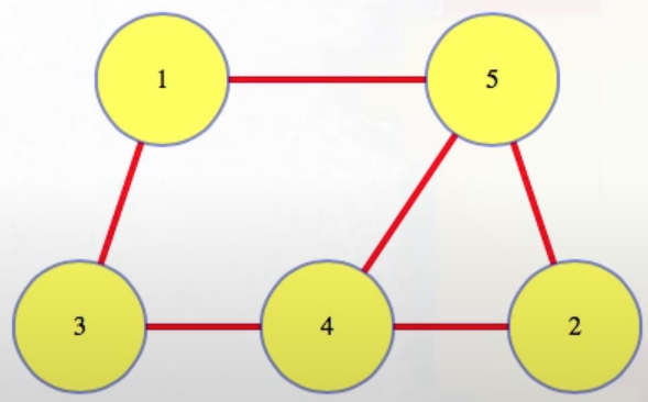
we get an adjacency matrix like the following:

$$\begin{array}{c|ccccc} {} & 1 & 2 & 3 & 4 & 5\\\hline 1 & \textcolor{blue}{\text{F}} & \text{F} & \color{red}{\text{T}} & \text{F} & \color{red}{\text{T}}\\ 2 & \text{F} & \textcolor{blue}{\text{F}} & \text{F} & \color{red}{\text{T}} & \color{red}{\text{T}}\\ 3 & \color{red}{\text{T}} & \text{F} & \textcolor{blue}{\text{F}} & \color{red}{\text{T}} & \text{F}\\ 4 & \text{F} & \color{red}{\text{T}} & \color{red}{\text{T}} & \textcolor{blue}{\text{F}} & \color{red}{\text{T}}\\ 5 & \color{red}{\text{T}} & \color{red}{\text{T}} & \text{F} & \color{red}{\text{T}} & \textcolor{blue}{\text{F}} \end{array}$$

Note that the matrix above is symmetric about the diagonal (top-left to bottom-right). So we could potentially try to halve our space by just keeping one side, namely the top half:

$$\begin{array}{c|ccccc} {} & 1 & 2 & 3 & 4 & 5\\\hline 1 & \textcolor{blue}{\text{F}} & \text{F} & \color{red}{\text{T}} & \text{F} & \color{red}{\text{T}}\\ 2 & {} & \textcolor{blue}{\text{F}} & \text{F} & \color{red}{\text{T}} & \color{red}{\text{T}}\\ 3 & {} & {} & \textcolor{blue}{\text{F}} & \color{red}{\text{T}} & \text{F}\\ 4 & {} & {} & {} & \textcolor{blue}{\text{F}} & \color{red}{\text{T}}\\ 5 & {} & {} & {} & {} & \textcolor{blue}{\text{F}} \end{array}$$

Or the bottom half:

$$\begin{array}{c|ccccc} {} & 1 & 2 & 3 & 4 & 5\\\hline 1 & \textcolor{blue}{\text{F}} & {} & {} & {} & {}\\ 2 & \text{F} & \textcolor{blue}{\text{F}} & {} & {} & {}\\ 3 & \color{red}{\text{T}} & \text{F} & \textcolor{blue}{\text{F}} & {} & {}\\ 4 & \text{F} & \color{red}{\text{T}} & \color{red}{\text{T}} & \textcolor{blue}{\text{F}} & {}\\ 5 & \color{red}{\text{T}} & \color{red}{\text{T}} & \text{F} & \color{red}{\text{T}} & \textcolor{blue}{\text{F}} \end{array}$$

Some books like [21] mention keeping the top half, but an argument can be made that the indices come out cleaner by keeping the bottom half.

Adjacency list

For the adjacency list representation, we have an array/list of vertices, and for each vertex we have a list of its edges. In the simplest case, if our current vertex i has an edge to j, then maybe we only need to store that index j in i's list to mark that the edge exists. For example, the graph

could be said to have the following adjacency list:

$$\begin{align*} 1 &\rightarrow\quad 3,\; 5\\ 2 &\rightarrow\quad 4,\; 5\\ 3 &\rightarrow\quad 1\\ 4 &\rightarrow\quad 3\\ 5 &\rightarrow\quad 1,\; 4 \end{align*}$$

We can't get away with just a single true/false bit here. We have to identify the other vertex. For a weight graph, we can't just store weights. We also need an index or reference.

List variants

What do we use for lists? We can use any list, and if the graph doesn't change, then we could just use static arrays. If the graph never changes, and we frequently have to look up whether or not edges exist, then we could even use sorted arrays and then just use binary search if we're looking for a particular vertex in the list. If we care about quick lookup and also want to let edges be added or removed, then we could even use a balanced binary tree structure.

But for lots of algorithms, we only look at all edges incident on a vertex in arbitrary order. For that, just about everything we might want to use is fine (dynamic arrays are often the structure of choice).

Undirected adjacency lists

For undirected graphs like

we store each edge twice when using the adjacency list model (once in the list for each vertex):

$$\begin{align*} 1 &\rightarrow\quad \color{red}{3},\; \color{blue}{5}\\ 2 &\rightarrow\quad {\color{green}{4}},\; 5\\ 3 &\rightarrow\quad \color{red}{1},\; \color{cyan}{4}\\ 4 &\rightarrow\quad \color{green}{2},\; \color{cyan}{3},\; \color{orange}{5}\\ 5 &\rightarrow\quad {\color{blue}{1}},\; 2,\; \color{orange}{4} \end{align*}$$

Outgoing and incoming lists

For directed graphs, we have a choice. For each vertex, we can store all the vertices that it has an edge to or all the vertices that it has an edge from.

Hence, for the directed graph

we would have the following as the vertex outgoing list (this is what was shown previously):

$$\begin{align*} 1 &\rightarrow\quad 3,\; 5\\ 2 &\rightarrow\quad 4,\; 5\\ 3 &\rightarrow\quad 1\\ 4 &\rightarrow\quad 3\\ 5 &\rightarrow\quad 1,\; 4 \end{align*}$$

Or we would have the following as the vertex incoming list:

$$\begin{align*} 1 &\leftarrow\quad 3,\; 5\\ 2 &\leftarrow\quad {}\\ 3 &\leftarrow\quad 1,\; 4\\ 4 &\leftarrow\quad 2,\; 5\\ 5 &\leftarrow\quad 1,\; 2 \end{align*}$$

These are two different ways of storing the same graph. We pick one representation over the other depending on how we're going to need to access our data. Storing outgoing edges is more common, but for some problems we may want both representations.

Transformations between lists

What if we're given the graph as an outgoing adjacency list, but we want the incoming list? We can go from one format to the other in time linear in the size of the graph. Given an outgoing representation, we create a new incoming representation with the same vertices, and then for each vertex i in the graph, and for each j in i's outgoing list, append i to j's incoming list:

for each vertex i
    for each outgoing edge (i, j)
        append i to j's incoming list

Going from the incoming list to the outgoing list uses the same approach.

Transforming adjacency list to adjacency matrix

Going from an adjacency list to an adjacency matrix is very similar:

create matrix
for each vertex i
    for each outgoing edge (i, j)
        mark matrix[i, j]

Transforming adjacency matrix to adjacency list

To go from an adjacency matrix to an adjacency list, we follow similar mechanics:

create outgoing representation with empty edge lists
for each (i, j) pair
    if (matrix[i, j] is an edge)
        append i to j's outgoing list

Graph transpose

One final graph manipulation algorithm: flipping the direction of each edge in a graph is called taking the graph's transpose because if we're using the adjacency matrix format, then we just take the transpose of the matrix:

for i = 1 to |V| - 1
    for j = i + 1 to |V|
        tmp = matrix[i, j]
        matrix[i, j] = matrix[j, i]
        matrix[j, i] = tmp

If we're using the outgoing adjacency list format, then just find the incoming adjacency list for the same graph, and then interpret that incoming list as the outgoing list:

find matching incoming list
interpret it as an outgoing list

That's the transpose.

Representation comparison (space)

Let's assume we have whatever graph representation we want for our problem at hand. Let's compare the outgoing adjacency list and adjacency matrix representations so we can get a better idea as to when it might be more appropriate to use one over the other.

First, let's look at the space or memory usage. The adjacency list has one list for each vertex, and each edge shows up in one of the lists (or twice for undirected graphs). That's space linear in the size of the graph: $\Theta(|V| + |E|)$. The adjacency matrix, on the other hand, takes up size quadratic in the number of vertices: $\Theta(|V|^2)$. Is that bad? It depends on how dense the graph is. If the graph has enough edges, then the matrix could actually use up somewhat less space than the adjacency list, but for sparse graphs the adjacency list is asymptotically better.

Representation comparison (time)

What tasks does each representation do well? The most common basic graph operations are to ask what vertices are adjacency to a vertex and to ask if an edge between two vertices exists. Iterating through a list of vertices adjacent to a vertex is easy with an outgoing adjacency list. It takes time linear in the size of the list, which is the vertex's out-degree. The matrix format takes time linear in the total number of vertices in the graph. Again, this isn't bad if the graph is dense and the vertex has an edge to most other vertices. But it gets worse and worse the more sparse the graph is.

The adjacency matrix representation can tell us if an edge exists in constant time while the adjacency list representation takes time linear in the degree of one of the edge vertices to run a linear search. If we expect to do lots of these lookups and decide to have the lists sorted in arrays or trees, then each lookup will only take time logarithmic in the degree of the vertex, which might be small compared to the number of vertices. That might be worth doing sometimes, but for lots of nice algorithms we don't look up whether or not an edge exists. We only want to list vertices by adjacency. Even though we will occasionally use the adjacency matrix, the adjacency list is our default.

To recap:

• Iterate through neighbors of a vertex i
  • Adjacency list: $\Theta(\text{outdegree}(i))$
  • Adjacency matrix: $\Theta(|V|)$
• Check for edge $(i, j)$
  • Adjacency matrix: $\Theta(1)$
  • Outgoing adjacency list:
    • Linked list or unsorted array: $O(\text{outdegree}(i))$
    • Sorted array or tree: $O(\lg(\text{outdegree}(i)))$

Breadth first search (BFS)

Breadth first search (BFS) is conceptually simple, easy to implement, and worth understanding fully because many other algorithms may be viewed as minor modifications of BFS. A BFS can run on directed or undirected graphs, and we ignore any weights. We'll assume we're dealing with an adjacency list representation of the graph as input.

Basic idea

The basic idea behind BFS is that we have a starting vertex and we explore vertices in order of how many links they are away from this starting vertex. So first explore the starting vertex:

Then explore all vertices one link away (i.e., incident edges involving the start vertex and its immediate neighbors):

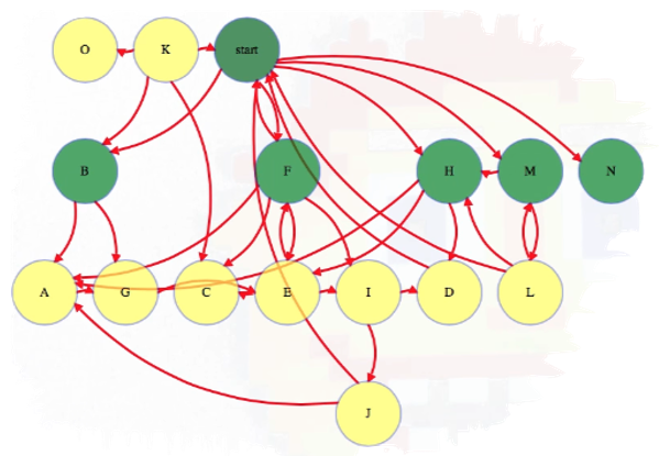
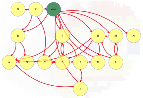
Then all vertices two links away:

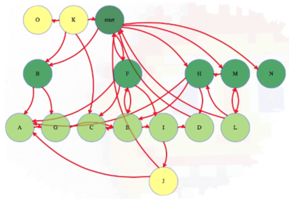
And so forth, until we have explored all vertices reachable from the start vertex:

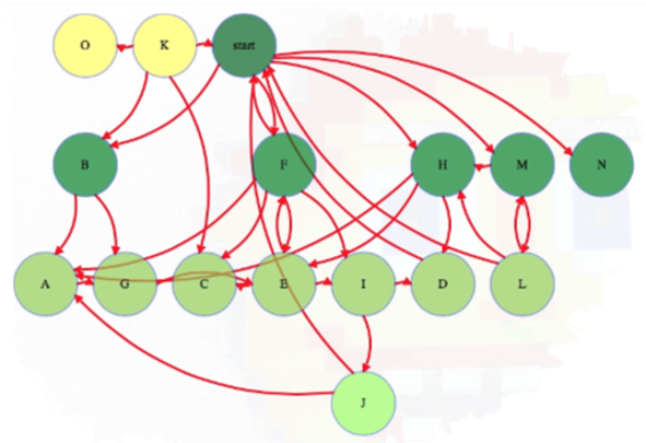
Above, each reachable vertex from the start vertex has an edge from the level above it but not from any higher reachable vertex. In this case, we have a couple of vertices that are not reachable from the start vertex, namely vertices O and K.

That's the whole concept. If we are looking for the shallowest of understandings, then we can stop there.

For the first visualization above, we started with vertices already in a position to easily see how many links they are from the start vertex. This may be helpful for humans in terms of readability, but a computer graph model does not need well-chosen locations for vertices — they're just abstractly positioned. We can put them wherever we like to visualize how the BFS is working.

For our simple BFS implementation, suppose we put them in a more arbitrary position:

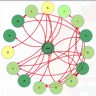
Now it's hard to really see what's going on in terms of how many links away from the start vertex each vertex is.

Simple imlpementation

Like with most graph algorithms, assume that each vertex has some room in it that the algorithm can use to store information. At the very least, the algorithm needs to mark each vertex as discovered or not.

• When the algorithm starts, we should initially mark all vertices as undiscovered (lines 1-3 in the pseudocode below).
• Next, mark the start vertex as discovered and push it into a first in first out queue (lines 7 and 9, respectively).
• After that, the algorithm is really just a simple loop. While the queue isn't empty (line 10), dequeue a vertex (line 11). For each of its outgoing edges (line 12), if they go to an undiscovered neighbor (line 13), then discover and enqueue the neighbor (lines 14 and 15, respectively).

The outline above provides everything we need for a simple BFS implementation:

ResetGraph()
    for v in V
        v.discovered = False

BFS(startVertex)
    ResetGraph()
    startVertex.discovered = True
    Q = new Queue()
    Q.enqueue(startVertex)
    while(not Q.isEmpty())
        u = Q.dequeue()
        for each v such that u -> v
            if(not v.discovered)
                v.discovered = True
                Q.enqueue(v)

The only thing the simple implementation above accomplishes is to mark the vertices which are reachable from the start vertex. Running this algorithm implies a specific so-called "BFS tree": the root is the start node, and if one node u discovers another node v, then node u is node v's parent in the BFS tree. For the same graph, we get a different BFS tree based on whatever node we pick as the start node. Things can get even wilder if we pick several start nodes, something that happens when executing a multi-source BFS.

Full implementation

A more detailed implementation of BFS would be as follows, where we not only create the BFS tree but also store the number of links needed to reach each vertex.

ResetGraph()
    for v in V
        v.discovered = False
        v.dist = inf
        v.pi = nil

BFS(startVertex)
    ResetGraph()
    startVertex.discovered = True
    startVertex.dist = 0
    Q = new Queue()
    Q.enqueue(startVertex)
    while(not Q.isEmpty())
        u = Q.dequeue()
        for each v such that u -> v
            if(not v.discovered)
                v.discovered = True
                v.dist = u.dist + 1
                v.pi = u
                Q.enqueue(v)

Of course, for the scheme above to work, assume there's space to store extra information with each vertex, v, namely the distance needed to reach the vertex as well as well as the predecessor parent for that vertex, v.dist and v.pi, respectively (lines 4 and 5 above, respectively). This information can be associated with the vertex itself so that we end up representing a vertex basically as a list, where each slot represents, say, the vertex index, the distance to that vertex, and then the predecessor for that vertex: [v_index, v_dist, v_pred]. These items then get enqueued, dequeued, and updated accordingly. But it's more common to leave the vertex indices to themselves and to instead initialize dist and pred arrays both of length n, where n represents the total number of vertices in the graph (remember we're assuming the underlying graph is an adjacency list of index arrays, where nodes are labeled according to their index).

Certainly an observation worth making is that vertices with a smaller distance value must be dequeued and processed before any vertex with a greater distance value is dequeued and processed (this is a defining characteristic of BFS). Predecessor values are recorded in part to aid in the process of potentially reconstructing the shortest path from the start vertex to one of its reachable vertices.

Queue observation

Take another look at our first example graph where we conducted a BFS:

The start vertex is discoverd at zero links away from itself. Each subsequent time we discover a node, it gets discovered in one more link than the node that discovered it; hence, in the graph above, we see vertices B, F, H, M, and N are all 1 link away from the start vertex.

Notice that, as we continue visiting nodes, the queue only contains one or two different distances in it at a time. We will not add any distance 3 vertices (i.e., J) until we remove a distance 2 vertex from the queue, which only happens after all distance 1 vertices have been removed. As we continue processing nodes, we should indicate which node discovered it (line 19 in the pseudocode above). These values can be used to reconstruct shortest paths from the root to any vertex.

Reconstructing shortest paths

Recursive pseudocode

Reconstructing the shortest path from the start vertex, s, to a target node, t, can be done recursively as follows:

FindPath(s, t)
    if (s == t)
        return new List().add(t)
    if (t.pi == nil) # no path exists
        return nil
    return FindPath(s, t.pi).add(t)

Iterative pseudocode

This can also be done iteratively (perhaps more intuitively), where the implementation below assumes we've maintained a pred array where pred[x] houses the predecessor for node x if it exists or is -1 otherwise:

ReconstructPath(s, t, pred)
    path = new Stack()
    path.push(t)
    while path.peek() != s:
        if pred[path.peek()] == -1:
            return NIL                  # no path exists from s to t
        path.push(pred[path.peek()])
    reverse path                        # obtain original path direction from s to t
    return path

Python implementations

In CLRS (i.e., [21]), the PrintPath procedure is provided to simply print the path from the vertex s to the vertex v (i.e., as opposed to really reconstructing the path):

PrintPath(G, s, v)
    if v == s:
        print s
    else if v.pi == nil:
        print "no path from" s "to" v "exists
    else PrintPath(G, s, v.pi)
        print v

We can use Python to implement the PrintPath procedure but in a way where we actually obtain the shortest path in a recursive manner:

Recursively reconstruct shortest path (Python)

def shortest_path(s, t, path, pred):
    if s == t:
        path.append(s)
        return path
    elif pred[t] == -1:
        return []  # shortest path from s to t does not exist
    else:
        path.append(t)
        return shortest_path(s, pred[t], path, pred)

In most cases, however, we would probably be more inclined to reconstruct the path in an iterative fashion, where the code is more readable and we avoid some of the overhead associated with recursion:

Iteratively reconstruct shortest path (Python)

def shortest_path(s, t, pred):
    path = [t]
    while path[-1] != s:
        parent = pred[path[-1]]
        if parent == -1:
            return []  # shortest path from s to t does not exist
        path.append(parent)
    path.reverse()
    return path

Cormen colors

If we look at [21], we will note that there's only a minor change from the "full implementation" algorithm above and how it appears in CLRS: instead of marking vertices as discovered or undiscovered, they use three colors:

• White: Undiscovered
• Gray: Discovered but not yet finished (i.e., when it's in the queue waiting to be dequeued)
• Black: Finished (i.e., dequeued and all unvisited child nodes enqueued)

That's it:

Full implementation of BFS (CLRS style)

ResetGraph()
    for v in V
        v.color = White
        v.dist = +inf
        v.pi = nil

BFS(startVertex)
    ResetGraph()
    startVertex.color = Gray
    startVertex.dist = 0
    Q = new Queue()
    Q.enqueue(startVertex)
    while(not Q.isEmpty())
        u = Q.dequeue()
        for each v such that u -> v
            if(v.color == White)
                v.color = Gray
                v.dist = u.dist + 1
                v.pi = u
                Q.enqueue(v)
        u.color = Black

Analysis

The initialization ResetGraph takes time linear in the number of vertices in the graph: $\Theta(|V|)$. After this, each reachable vertex can only be discovered and enqueued once. A vertex's outgoing edges only get explored when it's dequeued, which will also only happen once, and takes time proportional to the number of outgoing edges for that vertex (i.e., if we're using the adjacency list representation of a graph).

If we let $V'$ and $E'$ be the sets of vertices and edges reachable from the start vertex, respectively, then we have the following:

• $\Theta(|V'|)$ vertices discovered, enqueued, and dequeued.
• $\Theta(|E'|)$ edges explored by dequeued vertices.

For an undirected graph, reachable edges can be explored once from each side, but that still gives us a total linear time in the number of reachable vertices and edges. Thus, the total runtime may be characterized more precisely as $\Theta(|V'| + |E'|)$ or less optimistically as $O(|V| + |E|)$.

Handwavey correctness outline

If we really want to understand the correctness of BFS, then working out the details for ourselves will probably be our best bet. It't also not a bad idea to consult [21] or any other number of quality resources.

But let's give a thumbnail sketch. The first thing we need to know is what the BFS algorithm actually achieves. Informally, we have the following:

• For all vertices reachable from the start vertex:
  • Marks as discovered
  • Calculates minimum number of links from start vertex
  • Calculates predecessor on some minimum link path from start vertex (nil predecessor for start vertex)
• For vertices not reachable from the start vertex:
  • Marks as not discovered
  • Calculates distance as $\infty$
  • Gives nil predecessor

What does the algorithm do mechanically though? How does it operate? Here are a couple statements that can help:

• Set of vertices in $Q$ never has more than 2 distinct distances, one apart. Values enter and exit $Q$ in non-decreasing distance order. (To prove: induct on $Q$ contents.)
• All reachable vertices will be discovered, enqueued, marked with correct minimum link distances, and valid predecessor nodes (except the start vertex), which are never changed again. (To prove: Induction on edge count from start node).

Depth first search (DFS)

Depth-first search (DFS) on general graphs is conceptually simple and easy to implement, but it's worth understanding fully because several more advanced graph algorithms may be considered to be just minor modifications or extensions of DFS.

Basic idea

If we're looking at a graph from above, then breadth first search (BFS) is pretty intuitive. It expands from our search vertex like a wave in a pond:

0 links away from start node

1 / 4

But lots of times we're not looking at a graph from above — we're looking at it from within (e.g., we're exploring a maze, an area in a video game, etc.).

Or we could be watching the video on YouTube on which this section is based. We could model the video page as a vertex. If there are a bunch of video recommendations listed off to one side, then those links are like edges to other vertices. If we see three recommendations that look interesting, then maybe we click on one. From this second video, maybe we see four more recommended videos that look good. Do we click one of them? Or do we stop, remember that they're there, but then go back to the second video we were just at? Maybe we just keep clicking through our recommended videos until there aren't anymore to click through (unlikely!).

The process described above is like depth first search (DFS). If we go back and watch videos in the order in which we first saw a link to them, then that is like breadth first search. In this context, BFS would be harder to do unless we used something like tabs or a "watch later" list which would essentially work as the first-in-first-out queue in BFS.

For DFS, we just keep clicking on stuff, and when we run out of new stuff we want to see, then we hit the "Back" button on our browser to get back to the previous video.

Simple implementation

If we start thinking about what a simple implementation for DFS might look like, we can come up with something that is somewhat similar to the simple implementation for BFS:

ResetGraph(G)
    for v in V
        v.discovered = False
  
DFSVertex(u)
    u.discovered = True
    for each v such that u -> v
        if (not v.discovered)
            DFSVertex(v)

DFS(G, startVertex)
    ResetGraph(G)
    DFSVertex(startVertex)

To illustrate how the pseudocode above would work for a sample graph, consider the following partial traversal where the DFS starts at node I and then travels along the path I -> E -> H -> D -> B -> A:

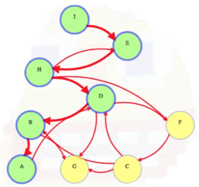
Worth noting is that if we start at node I, then we have no choice but to go to node E next. We then have to go to node H. But once we're at H, we can either go to node D or to node F. The order does not matter because we will end up visiting both D and F. We arbitrarily choose D (oftentimes we'll just choose to visit neighboring nodes in alphabetical order for the sake of clarity and consistency). The important point: We start from a single vertex and then go to adjacent vertices. If the next vertex has several adjacent vertices (e.g., like D and F for node H discussed above), it doesn't matter — we just choose one of them and keep exploring, ignoring other vertices we could have explored along the way. We do this by making recursive calls to DFSVertex for each new vertex:

DFSVertex(I)
    DFSVertex(E)
        DFSVertex(H)
            DFSVertex(D)
                DFSVertex(B)
                    DFSVertex(A)

Once we call DFSVertex(A) above, we see that the only outgoing edge from vertex A is to vertex D. But we've already visited or "discovered" vertex D, and we don't want to visit it again. Hence, we exit A's DFSVertex call, returning to B (i.e., we backtrack to vertex B from A). When we first called DFSVertex(B), we were looping through B's outgoing edges to see which vertices to visit next when it made the call to search A, but now that A is done being searched, B's loop resumes and it requires us to explore its edge to G. Vertex G has no outgoing edges so it finishes. Then B finishes. Then control goes back to D. Now that D's call to B is finished, D's loop resumes, and it searches F. And so on:

DFSVertex(I)
    DFSVertex(E)
        DFSVertex(H)
            DFSVertex(D)
                DFSVertex(B)
                    DFSVertex(A)
                    DFSVertex(G)
                DFSVertex(F)
                    DFSVertex(C)

In BFS, D and F would both be children of H. Like in BFS, if we think about what vertex discovers another, then this implies the existence of some sort of "DFS tree" rooted at the initial search vertex. In the example graph we've been considering, this would mean we have a DFS tree rooted at vertex I (tree edges are highlighted with thicker directed red edges):

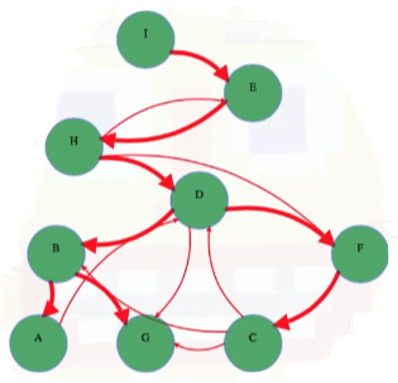
We can update our simple implementation pseudocode to store parent values in a $\pi$ variable (to further explore properties of the DFS tree):

ResetGraph(G)
    for v in V
        v.pi = nil
        v.discovered = False
  
DFSVertex(u)
    u.discovered = True
    for each v such that u -> v
        if (not v.discovered)
            v.pi = u
            DFSVertex(v)

DFS(G, startVertex)
    ResetGraph(G)
    DFSVertex(startVertex)

Full implementation

Similar to BFS, in DFS we can reconstruct paths from the root of the tree — but the paths are less interesting here because they might have more than the minimum number of links. So instead of counting links, we track when each vertex was discovered (i.e., reached) and finished (i.e., fully explored) with "timestamps". Of course, we don't need actual timestamps — just a relative order will do:

ResetGraph(G)
    for v in V
        v.pi = nil
        v.discovered = -1
        v.finished = -1
    time = 1
  
DFSVertex(u)
    u.discovered = time++
    for each v such that u -> v
        if (v.discovered < 0)
            v.pi = u
            DFSVertex(v)
    u.finished = time++

DFS(G, startVertex)
    ResetGraph(G)
    DFSVertex(startVertex)

At this point, it may be worth reproducing the pseudocode from [21] to serve as a comparison point in terms of how nodes are tracked and managed. Specifically, CLRS uses not only timestamps but also colors as well (similar to what was used for BFS):

• White: Undiscovered
• Gray: Discovered but not yet finished (i.e., it is actively being explored)
• Black: Finished (i.e., it is done being explored)

With the above in mind, here is the DFS algorithm as it appears in CLRS:

CLRS implementation of DFS

DFS(G)
    for each vertex u in G.V
        u.color = White
        u.pi = nil
    time = 0
    for each vertex u in G.V
        if u.color == White
            DFSVisit(G, u)

DFSVisit(G, u)
    time = time + 1                 # white vertex has just been discovered
    u.d = time
    u.color = Gray
    for each vertex v in G.Adj[u]   # explore each edge (u, v)
        if v.color == White
            v.pi = u
            DFSVisit(G, v)
    time = time + 1
    u.f = time
    u.color = Black                 # blacken u; it is finished

Why would we want to track timestamps when executing a DFS? It turns out that DFS timestamps will be useful for other tasks and algorithms (e.g., topological sorting, finding strongly connected components (SCCs), etc.).

Vertex vs. graph DFS

For some algorithms, we want to run DFS from one vertex (e.g., maybe we're interested in knowing what other vertices can be reached from this vertex) while for others we want to run it on the whole graph (i.e., we want to search all vertices).

To do this, after initializing the graph once (i.e., with ResetGraph), we can run DFS on each previously undiscovered vertex; then, instead of getting a DFS tree rooted at one vertex (i.e., startVertex) that only includes vertices reachable from that vertex, we get a DFS forest comprised of several DFS trees that will always contain all the graph's vertices.

In terms of our earlier pseudocode for the full implementation, this means making the following change:

DFS on a single vertex

DFS(G, startVertex)
    ResetGraph(G)
    DFSVertex(startVertex)

DFS on all vertices (the entire graph)

DFS(G)
    ResetGraph(G)
    for u in V
        if (u.discovered < 0)
            DFSVertex(u)

We then get the following as our updated full implementation:

ResetGraph(G)
    for v in V
        v.pi = nil
        v.discovered = -1
        v.finished = -1
    time = 1
  
DFSVertex(u)
    u.discovered = time++
    for each v such that u -> v
        if (v.discovered < 0)
            v.pi = u
            DFSVertex(v)
    u.finished = time++

DFS(G)
  ResetGraph(G)
  for u in V
      if (u.discovered < 0)
          DFSVertex(u)

Example

It's a useful exercise to consider an example graph and work out how everything above is represented and calculated. To that end let's consider an example of the algorithm above in action on the following graph:

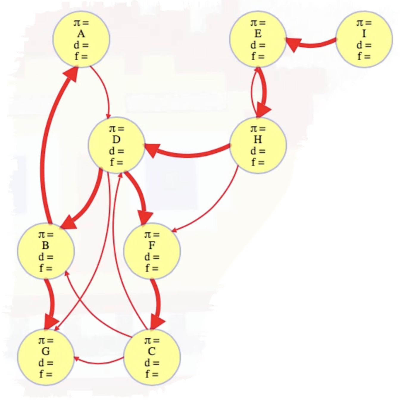
We'll execute top-level DFS searches on vertices in alphabetical order. Doing so yields the following completely searched graph:

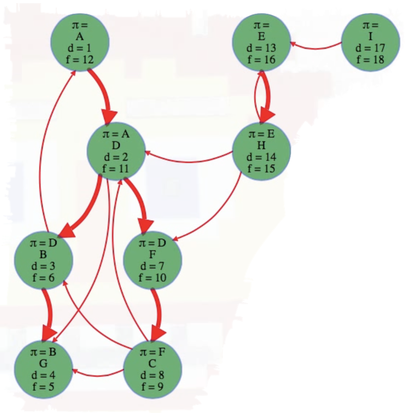
As can be seen above, A, E, and I are the roots of their own depth first search trees in this DFS forest.

To reproduce the final figure above using code, we can first represent the graph by mapping vertices A through I to 0 through 8, inclusive. It also helps to define a lookup table for ease of reference:

graph = [
    [3],
    [0, 6],
    [1, 3, 6],
    [1, 5, 6],
    [7],
    [2],
    [],
    [3, 4, 5],
    [4],
]

lookup = {
    -1: ' ',
    0: 'A',
    1: 'B',
    2: 'C',
    3: 'D',
    4: 'E',
    5: 'F',
    6: 'G',
    7: 'H',
    8: 'I',
}

Now we can write the dfs function to execute a DFS on the entire graph — the inner visit function is where the DFSVertex method is implemented (a reformatting of the output is included at the bottom of the code for ease of reference):

def dfs(graph):
    n = len(graph)
    discovered = [-1] * n
    finished = [-1] * n
    pred = [-1] * n
    time = 0
    
    def visit(node):
        nonlocal time
        time += 1
        discovered[node] = time
        for nbr in graph[node]:
            if discovered[nbr] < 0:
                pred[nbr] = node
                visit(nbr)
        time += 1
        finished[node] = time
        
    for node in range(n):
        if discovered[node] < 0:
            visit(node)
            
    return discovered, finished, [ lookup[parent] for parent in pred ]

print(dfs(graph))

""" 

(     A  B  C   D   E   F  G   H   I
    [ 1, 3, 8,  2, 13,  7, 4, 14, 17],  # discovered times
    [12, 6, 9, 11, 16, 10, 5, 15, 18],  # finished times
    [  , D, F,  A,   ,  D, B,  E,   ]   # pi values
)

"""        

Note that the roots of the trees in the DFS forest (i.e., A, E, and I) do not have $\pi$-values, as expected. Try the code above yourself to confirm what's been described (feel free to tweak the code and experiment):

Loading...

Output

Click "Run Code" to see the output here

The next two aspects of DFS we will consider, namely parenthesis notation and edge classification, are remarked on in greater detail in [21]. The relevant snippets from CLRS are reproduced below (it would likely be helpful to look at these snippets before looking at these topics in the context of the example we've been working through).

Parenthesis theorem (CLRS)

Depth-first search yields valuable information about the structure of a graph. Perhaps the most basic property of depth-first search is that the predecessor subgraph $G_\pi$ does indeed form a forest of trees, since the structure of the depth-first trees exactly mirrors the structure of recursive calls of DFS-VISIT. That is, $u = v.\pi$ if and only if $\text{DFS-Visit}(G, v)$ was called during a search of $u$'s adjacency list. Additionally, vertex $v$ is a descendant of vertex $u$ in the depth-first forest if and only if $v$ is discovered during the time in which $u$ is gray.

Another important property of depth-first search is that discovery and finish times have parenthesis structure. If the DFS-VISIT procedure were to print a left parenthesis "$(u$" when it discovers vertex $u$ and to print a right parenthesis "$u)$" when it finishes $u$, then the printed expression would be well formed in the sense that the parentheses are properly nested.

The following theorem provides another way to characterize the parenthesis structure.

In any depth-first search of a (directed or undirected) graph $G = (V, E)$, for any two vertices $u$ and $v$, exactly one of the following three conditions holds:

• the intervals $[u.d, u.f]$ and $[v.d, v.f]$ are entirely disjoint, and neither $u$ nor $v$ is a descendant of the other in the depth-first forest,
• the interval $[u.d, u.f]$ is contained entirely within the interval $[v.d, v.f]$, and $u$ is a descendant of $v$ in a depth-first tree, or
• the interval $[v.d, v.f]$ is contained entirely within the interval $[u.d, u.f]$, and $v$ is a descendant of $u$ in a depth-first tree.

Edge classification (CLRS)

You can obtain important information about a graph by classifying its edges during a depth-first search. For example, Section 20.4 will show that a directed graph is acyclic if and only if a depth-first search yields no "back" edges (Lemma 20.11).

The depth-first forest $G_\pi$ produced by a depth-first search on graph $G$ can contain four types of edges

1. Tree edges are edges in the depth-first forest $G_\pi$. Edge $(u, v)$ is a tree edge if $v$ was first discovered by exploring edge $(u, v)$.
2. Back edges are those edges $(u, v)$ connecting a vertex $u$ to an ancestor $v$ in a depth-first tree. We consider self-loops, which may occur in directed graphs, to be back edges.
3. Forward edges are those nontree edges $(u, v)$ connecting a vertex $u$ to a proper descendant $v$ in a depth-first tree. [If $y$ is an ancestor of $x$ and $x\neq y$, then $y$ is a proper ancestor of $x$ and $x$ is a proper descendant of $y$.]
4. Cross edges are all other edges. They can go between vertices in the same depth-first tree, as long as one vertex is not an ancestor of the other, or they can go between vertices in different depth-first trees.

The DFS algorithm has enough information to classify some edges as it encounters them. The key idea is that when an edge $(u, v)$ is first explored, the color of vertex $v$ says something about the edge:

1. WHITE indicates a tree edge,
2. GRAY indicates a back edge, and
3. BLACK indicates a forward or cross edge.

The first case is immediate from the specification of the algorithm. For the second case, observe that the gray vertices always form a linear chain of descendants corresponding to the stack of active DFS-VISIT invocations. The number of gray vertices is 1 more than the depth in the depth-first forest of the vertex most recently discovered. Depth-first search always explores from the deepest gray vertex, so that an edge that reaches another gray vertex has reached an ancestor. The third case handles the remaining possibility.

Parenthesis notation

The entire depth first search from the worked example above can be summarized nicely using parentheses:

An opening parenthesis denotes when the DFS call is made on a vertex, and the closed parenthesis stands for when that call exits:

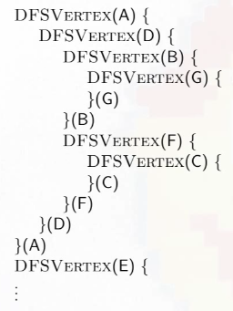
The parentheses are properly nested because the inner recursive calls must complete before the code that called them. A child will always be nested in its parent, and a vertex is only the child of at most one vertex, the one that discovered it.

If we just count the parentheses from the beginning, then they will match the discovery and finish times noted previously:

We can also see how each DFS tree of the DFS forest naturally corresponds to sets of parentheses delimited by an opening parenthesis for where the search started (i.e., the root of a DFS tree) and the corresponding closed parenthesis when the search for that vertex has ended:

The parenthesis method outlined above may seem odd at first, but it really provides a nice way of looking at how a DFS works manually (for small graphs).

Cormen vertex colors

Recall the fully explored graph for reference and comparison:

In CLRS they do two more things than what we've been doing thus far. First, they color vertices in the following manner:

• White: Undiscovered
• Gray: Discovered (but unifinished)
• Black: Finished

Edge classifications

The second thing CLRS does is classify edges into tree-edges (i.e., edges directly part of a DFS tree) and three types of non-tree edges (i.e., edges that exist in the graph but are not part of the DFS tree). For the edge classification descriptions that follow, it will help if we first provide some notational shorthand to make our ideas and descriptions precise:

• Vertex labels: Let u and v be the endpoints of the edge u -> v under consideration. We will then flesh out what it means for the edge u -> v to be a tree edge, back edge, forward edge, or cross edge.
• Discovery and finishing times: Let u.d, u.f, v.d, and v.f denote the discovery and finishing times of vertices u and v, respectively. Let -1 denote missing values; that is, if vertex x has not yet been discovered, then x.d = -1. Similarly, if vertex x has not been finished, then x.f = -1.

We can now discuss the various edge classifications effectively. With the list that follows, it helps to think about approaching the classifications in an ordered manner; that is, we progressively ask ourselves if u -> v is a tree edge (v.d == -1), a back edge (v.f == -1), a forward edge (v.d > u.d), or a cross edge (v.f < u.d or u.f < v.d, but anything here flies since none of the previous conditionals hold):

• Tree edges (parent to a child): go to an undiscovered vertex

  Mathematically: v.d == -1. If we reach an undiscovered vertex v from vertex u, then u -> v is a tree edge; that is, u discovers v as a direct child (u is an ancestor and v is a direct descendant — it's a parent/child relationship).

• Back edges (to an ancestor): to a discovered but unfinished vertex (creates a cycle)

  In a nutshell, the edge u -> v is a back edge if vertex u goes back to some previously discovered yet unfinished vertex v.

  More thoroughly, a back edge u -> x is an edge from vertex u to its ancestor x (e.g., its parent, or grandparent, or further up). From the ancestor x there's a path of tree edges from x leading to vertex u. Adding the back edge u -> x to those tree edges makes a cycle. Without looking at the graph picture as a whole, how could we tell locally while we look at the edge u -> x that x is an ancestor of u? In the context of our graph, how can we tell that vertex A is an ancestor of vertex B? Because A has already been discovered, but it isn't finished yet. A's parentheses are still open, and A can't finish until after the current vertex B does. So A's parentheses must surround those of B's, and thus it's B's ancestor. So B -> A is a back edge. During a DFS, every back edge completes a cycle. Removing all back edges from a graph would remove all cycles.

  It's also worth noting that a self-edge (i.e., an edge from a vertex to itself) is considered to be a back edge to be consistent with our terminology: it completes a cycle (of length 1), and it goes to a vertex that's been discovered but not yet finished at the time we explore the self-edge.

  Mathematically: v.f == -1. If v.d != -1, then we know v has already been discovered and thus u -> v cannot be a tree edge. If we somehow got to vertex u from vertex v by following a path of tree edges from vertex v to vertex u, then it's clear that vertex v has not yet been finished. The edge u -> v closes the loop (creates a cycle). Note that we could update the condition to be v.d < u.d and v.f != -1 in order to emphasize the fact that v was discovered before u, but not yet finished, which is why u -> v creates a cycle. The condition v.d < u.d is implied and thus not strictly necessary.

• Forward edges (to a non-child descendant): to a finished vertex discovered after the current vertex

  A forward edge is basically an edge that goes to an indirect descendant, not a direct child. For the graph we've been considering, the edge from D to G is a forward edge. How can we tell? Because G is finished but its discovery time is after that of the current node, D. The vertex G was discovered and explored during the lifetime of G — it's a descendant of D but not a direct descendant. Node B is the direct descendant of D; node G is the direct descendant of B; and node G is an indirect descendant of D. A forward edge goes to an indirect descendant, not a direct child (otherwise it would be a tree edge).

  Mathematically: v.d > u.d. If the edge is neither a tree edge nor a back edge, but we somehow still got directly from u to v via the edge u -> v, then it's clear the discovery time of v must be after the discovery time of u. So vertex v is, indeed, a descendant of u but only in an indirect way — if v were a direct descendant of u in the DFS tree, then u -> v would be a tree edge and would have been accounted for in the previous conditional checks. But if we wanted to mathematically distinguish forward edges from tree edges (since v.d > u.d for both) without relying on "previous conditional checks" to do the trick, then we need to ensure v has already been discovered and finished by the time it is reached by u (i.e., v is a descendant of u but not reached via u -> v). Mathematically, this condition could be expressed as u.d < v.d and u.f > v.f and v.d != -1 (i.e., v is already discovered and finished when exploring u); this ensures v is a descendant of u (u.d < v.d and u.f > v.f) but not via a tree edge.

• Cross edges (everything else): to a vertex finished before the current vertex's discovery. It's essentially any edge that's not captured in the edge classifications above. It can go from one branch of a tree to another or even from one tree to another. And there isn't any ancestor or descendant relation between the vertices it links. You can tell because it leads to a vertex that finished before the current vertex was discovered. Its parentheses don't overlap.

  Mathematically: v.f < u.d or u.f < v.d. Cross edges occur between nodes that have no ancestor-descendant relationship, which means their discovery and finish times do not overlap; that is, the intervals [v.d, v.f] and [u.d, u.f] are disjoint. This can be expressed mathematically with the condition v.f < u.d or u.f < v.d. But ultimately there's no need to test this explicitly here if we're relying on the previous edges to be identified first —the "cross edge" label is more like a bucket: it holds all edges that cannot be classified as tree, back, or forward edges. We'll classify an edge as a cross edge no matter what if all previous tests for the other edges fail.

Everything above can be described quite simply in terms of vertex colors:

• Tree edge: Leads to a white vertex.
• Back edge: Leads to a gray vertex.
• Forward/cross edge: Leads to a black vertex.

If we color our example graph so that tree edges are red, back edges are black, forward edges are blue, and cross edges are green, then we end up with the following:

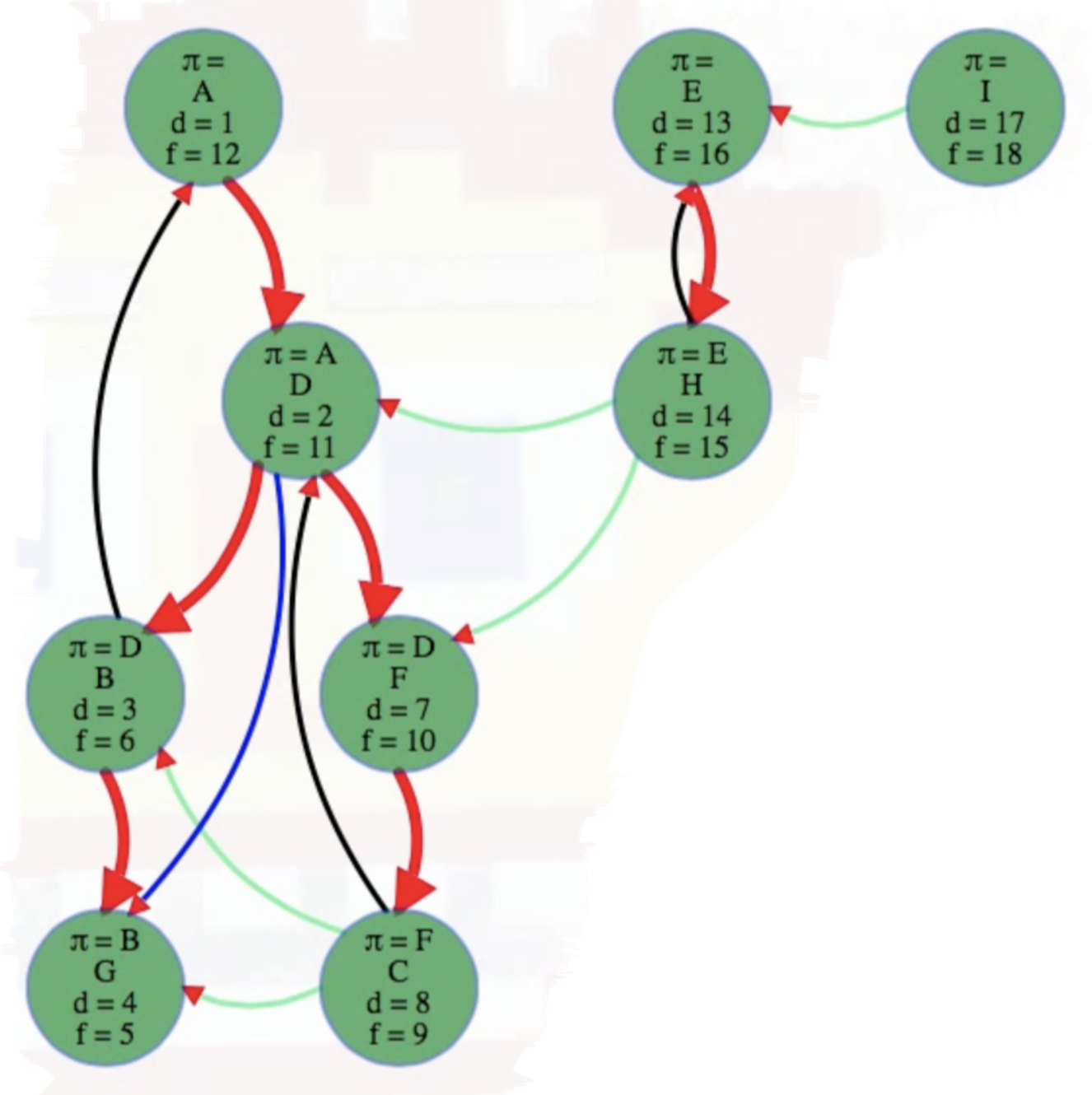
The edge classifications discussed above are meant to be understood in the context of directed graphs. What about undirected graphs? If the graph is undirected, then we end up seeing each edge twice, once from each vertex. If we classify the edge the first time we see it, then there won't be any forward or cross edges, only tree and back edges.

Analysis

Analysis of DFS is not too bad. If we run DFS on the entire graph, then we loop through all vertices but only call DFS once on each vertex in total. We explore every edge once (or twice in undirected graphs), and it takes time linear in the graph size: $\Theta(|V| + |E|)$. If we run DFS on just a single vertex, then it takes time linear in all vertices to initialize but then time linear in just the reachable portion of the graph: $\Theta(|V'| + |E'|)$, where $V'$ and $E'$ are the reachable vertices and edges from the source node, respectively.

Concern for potential stack overflow

Unlike BFS, if a graph is more connected, then its DFS trees tend to be taller and more vine-like. If vertices have lots of outgoing edges, then you can keep finding new vertices to explore, and the tree depth can get large. This brings us to a possible implementation hiccup for DFS — for each recursive call, we push variables onto our program's call stack. Different languages have different limits to how deep the call stack can be. A graph with 20,000 vertices might try to make 20,000 nested recursive DFS calls, which can give you a program stack overflow error. To avoid this, we can use our own stack instead of the implicit call stack with recursion.

Iterative DFS with a stack

We can do this in a few ways, but here is one possible manner (note: in general, we need to be cautious when implementing iterative DFS with a stack because we may end up with a "fake" DFS tree if we're not careful):

Non-recursive DFS

ResetGraph(G)
    for v in V
        v.pi = nil
        v.discovered = -1
        v.finished = -1
    time = 1
    
ExploreVertex(u, S)
    if (u.discovered < 0)
        u.discovered = time++
        S.push(u)
        for each v such that u -> v
            S.push(u -> v)
    else if (u.finished < 0)
        u.finished = time++
    # else: ignore, top level search of finished vertex

ExploreEdge(u -> v, S)
    if (v.discovered < 0)
        (u -> v).label = "treeEdge"
        v.pi = u
        ExploreVertex(v, S)
    else if (v.finished < 0)
        (u -> v).label = "backEdge
    else if (v.discovered > u.discovered)
        (u -> v).label = "forwardEdge"
    else
        (u -> v).label = "crossEdge"

DFS(G)
    ResetGraph(G)
    S = new Stack()
    for u in V
        S.push(u)
    while (not S.isEmpty())
        x = S.pop()
        if (x.isVertex())
            ExploreVertex(x, S)
        else
            ExploreEdge(x, S)

Let's go through how the pseudocode above is meant to function:

• Line 32: Here, we make a stack where we can push edges and vertices (we push edges in order to classify them).
• Lines 33-36: Push all vertices on to the stack and pop while the stack isn't empty.
• Lines 9-13: If we pop an undiscovered vertex, then discover it! Push it again to finish it later, and push its outgoing edges. When we pop it again later, after it's discovered (line 14), then finish it (line 15). And if we pop an already finished vertex, then just ignore it (line 16). That's the equivalent of looping through all vertices but only running depth first search on the undiscovered ones.
• Lines 19-28: When we pop an edge from the stack, if it leads to an undiscovered vertex, then it's a tree edge and label it as so (line 20) and explore that vertex (line 22); otherwise, just label the edge (using the conditions discussed previously in the section on edge classifications) and we're done with it (lines 23-28).

In the two lines where we push either all vertices (line 34) or all edges from a vertex (line 13), if we push them in the opposite order that we would normally loop through them in the recursive version of the algorithm, then the version above will give us the same results, timestamps, edge classifications, etc. It will all be the same as the recursive version. The code above doesn't look quite as clean, but it's a nice parallel to see that while breadth first search explicitly uses a first in first out queue of vertices, depth first search can explicitly use a stack of vertices and edges instead of just implicitly using the program call stack.

If we implement all of the pseudocode above for the iterative version in Python, then we will end up with something like the following (the blocks of code have been highlighted where ordering has intentionally been reversed to ensure the same results as the recursive version):

def dfs_iter(graph):
    n = len(graph)
    edge_classifications = dict()
    discovered = [-1] * n
    finished = [-1] * n
    pred = [-1] * n
    time = 0
    
    def explore_vertex(node):
        nonlocal time
        if discovered[node] < 0:
            time += 1
            discovered[node] = time
            stack.append(node)
            for i in range(len(graph[node]) - 1, -1, -1):
                nbr = graph[node][i]
                stack.append((node, nbr))
        elif finished[node] < 0:
            time += 1
            finished[node] = time
    
    def explore_edge(edge):
        node, nbr = edge
        if discovered[nbr] < 0:
            edge_classifications[edge] = 'treeEdge'
            pred[nbr] = node
            explore_vertex(nbr)
        elif finished[nbr] < 0:
            edge_classifications[edge] = 'backEdge'
        elif discovered[nbr] > discovered[node]:
            edge_classifications[edge] = 'forwardEdge'
        else:
            edge_classifications[edge] = 'crossEdge'
            
    stack = []
    for node in range(n - 1, -1, -1):
        stack.append(node)
    
    while stack:
        x = stack.pop()
        if not isinstance(x, tuple):
            explore_vertex(x)
        else:
            explore_edge(x)
        
    return discovered, finished, pred, { (lookup[edge[0]], lookup[edge[1]]): edge_classifications[edge] for edge in edge_classifications }

The outcome, formatted manually for the sake of clarity, matches exactly what was produced previously using the recursive approach (the edge classification also matches what we would expect):

""" 

(     A  B  C   D   E   F  G   H   I
    [ 1, 3, 8,  2, 13,  7, 4, 14, 17],  # discovered
    [12, 6, 9, 11, 16, 10, 5, 15, 18],  # finished
    [-1, 3, 5,  0, -1,  3, 1,  4, -1],  # predecessors
    {                                   # edge classifications
        ('A', 'D'): 'treeEdge',
        ('D', 'B'): 'treeEdge',
        ('B', 'A'): 'backEdge',
        ('B', 'G'): 'treeEdge',
        ('D', 'F'): 'treeEdge',
        ('F', 'C'): 'treeEdge',
        ('C', 'B'): 'crossEdge',
        ('C', 'D'): 'backEdge',
        ('C', 'G'): 'crossEdge',
        ('D', 'G'): 'forwardEdge',
        ('E', 'H'): 'treeEdge',
        ('H', 'D'): 'crossEdge',
        ('H', 'E'): 'backEdge',
        ('H', 'F'): 'crossEdge',
        ('I', 'E'): 'crossEdge'
    }
)

"""

Try it for yourself to verify and/or experiment:

Loading...

Output

Click "Run Code" to see the output here

Why is the order reversal in the iterative version important in order to ensure the same results as in the recursive version? Because stacks are last in first out (LIFO) data structures — if we push elements onto the stack in the same order as we would process them recursively, then they will be popped off in reverse order. Consider the worked example we've been dealing with throughout this entire post. If we pushed the vertices A through I onto the stack in that order, then the first vertex popped off would be I, not A. But that's not the desired result! Hence, we push vertices I, H, ... , B, A onto the stack in that order so they are popped in the order A, B, ... , H, I, much as the order they are processed in the recursive version. Similarly, the order in which neighboring vertices are processed needs to be reversed as well; that is, we need to push neighbors onto the stack in reverse order — this ensures that when they are popped off the stack, they are processed in the original order.

Consider a generalized example to fully clarify things:

• Adjacency list: Let's say u has neighbors [v1, v2, v3].
• Recursive DFS: Processes v1, then v2, then v3.
• Iterative DFS (without reversal):
  • Push v1, v2, v3 onto the stack.
  • Pop and process v3, v2, v1 (reverse order).
• Iterative DFS (with reversal):
  • Push v3, v2, v1 onto the stack.
  • Pop and process v1, v2, v3 (original order).

---