Dynamic programming (with attitude)

October 1, 2024

Software Engineer

This post explores dynamic programming. As usual, the Fibonacci numbers are used to introduce several key components of dynamic programming. This sets the stage for more advanced dynamic programming problems: rod cutting, subset sum, and Floyd-Warshall.

Attribution

The notes below come from the Algorithms with Attitude YouTube channel, specifically the Dynamic Programming playlist comprised of the following videos: Introduction to Dynamic Programming: Fibonacci Numbers, Rod Cutting, Subset Sum, and Floyd-Warshall All-Pairs Shortest Paths: A Dynamic Programming Approach.

There are several sections in this post, accessible in the table of contents on the right, but most of the sections have been listed below for ease of reference and navigation.

Introduction to dynamic programming - Fibonacci numbers
The rod cutting problem
The subset sum problem
Floyd-Warshall

Introduction to dynamic programming - Fibonacci numbers

Fibonacci number definition

Let's go ahead and start with a definition of the Fibonacci numbers:

F_n = \begin{cases} 0 &\text{if } n=0 \\ 1 &\text{if } n=1 \\ F_{n-1} + F_{n-2} &\text{if } n > 1 \end{cases}

Simple recursive algorithm

Unsurprisingly, we can implement a simple recursive program to calculate the $i$ th Fibonacci number:

Fib(n) {
    if (n < 2)
        return n
    return Fib(n - 1) + Fib(n - 2)
}

And it works! But there's a problem. It's super slow. To see this for ourselves, consider the Python implementation below that uses the Piston API for code execution. We can calculte up to roughly the 33rd Fibonacci number, but it times out and chokes when trying to calculate the 34th Fibonacci number:

Output

Click "Run Code" to see the output here

As shown above, even calculating the 33rd Fibonacci number takes a good bit of time. It's certainly not quick.

Recursion tree

Let's take a look at the recursion tree for running Fib(8):

The call tree above reflects the order in which Fib calls were made; that is, if we make the call to the previous Fibonacci number first (i.e., Fib(n - 1)), then the left spine of the tree has length 7; similarly, each time we have a second recursive call, the value goes down by 2 instead of 1 (i.e., Fib(n - 2)); hence, the right spine of the tree will have length 4:

More generally, the right spine has length about $n/2$ so the top $n/2$ levels of the tree are complete; that is, each of the $n/2$ levels is a fully binary tree:

The tree has at least $2^{n/2}$ nodes, where each node represents a call to Fib. That's exponential. Hence, we have a runtime of $\omega(2^{n/2}) = \omega(\sqrt[n]{2})$ ; more precisely: $\Theta(((1+\sqrt{5})/2)^n)$ .

But there's hope. Note the two subtrees rooted at 5 in the middle of the tree:

These subtrees are exactly the same. We're just repeating the same work. Not only that but there's an another subtree rooted at 5 all the way on the left (left child of 6 on left spine). Every one of those subtrees computes the 5th Fibonacci number, and this number is always 5. It's kind of dumb to repeat all of that work three separate times. Subtrees rooted at 4 may be smaller, but it gets repeated five times!

This explains the motivation behind the first big idea of dynamic programming: remember the values you have recursively computed! So that you don't repeat any work.

Memoized algorithm

Fibonacci(n) {
    Allocate Ans[0...n] = NIL everywhere
    Ans[0] = 0
    Ans[1] = 1
    return Fib(n, Ans)
}

Fib(n, Ans[]) {
    if (Ans[n] == NIL)
        Ans[n] = Fib(n - 1, Ans) + Fib(n - 2, Ans)
    return Ans[n]
}

We can add a dummy wrapper Fibonacci (line 1) that allocates a table to hold all the values (line 2). And then we can just slightly change the main program to check the table for an answer before making any recursive calls (line 9). If the answer was not stored in the table, then make the recursive calls, but, critically, save the value (line 10) before returning it (line 11). We could have kept the same base cases as before, but we instead incorporated them directly into the tables (lines 3 and 4).

If we implement the new pseudocode above, then we see that calculating the 34th Fibonacci is no longer a problem. Even calculating something as large as the 300th Fibonacci number isn't an issue:

Output

Click "Run Code" to see the output here

Pruned recursion tree

What does the effect of "remembering recursively computed values" have on the recursion tree? Let's find out. Here's how our "remembering table" starts (a value of -1 represents a null value, and the base case values have been filled in):

The recursion tree starts filling out much as before:

Within the table, the recursive calls shown above in the recursion tree start from the right and keep moving left towards the base cases:

Once we actually get down to the base cases

the table starts filling in (from the left and in order):

In the recursion tree, the left spine looks exactly the same as before, and each of the first-time calls we make to compute the $i$ th value has a subtree:

But once we leave that spine, the second time we try to compute the $i$ th value, we just look up the answer without any recursive calls, essentially pruning that subtree down to just a leaf. For example, in the recursion tree shown above, suppose we've traveled down the spine, and we're working our way back up, and we're about to make the recursive call to fib(3) from fib(5):

But we've already computed the third Fibonacci number! Our lookup table allows us to compute fib(3) in constant time, making it possible for us to not repeat any work (i.e., the subtree to the right of fib(5) is pruned to just be a leaf now).

The process illustrated above is the main idea behind dynamic programming. It's not "programming by James Bond" — it gets its name partially from dynamic memory allocation used to store the recursive subproblem answers. The table that holds the recursive subproblem answers is like a well-organized bunch of post-it notes or memos. The method above is fittingly called memoization (not memorization). It allows us to keep the same natural recursive structure of our code, but it keeps us from recomputing values.

Alternate version (order of recursively computed values)

It's worth looking at a very slightly different version of the program with just a switch in the order of our recursive calls:

Original program
Fib(n) {
    if (n < 2)
        return n
    return Fib(n - 1) + Fib(n - 2)
}

Altered program
Fib(n) {
    if (n < 2)
        return n
    return Fib(n - 2) + Fib(n - 1)
}

What happens to the recursion tree? For the un-memoized version, it looks the same as before, except that now the long spine is on the right:

But for the memoized version, the tree will actually look different (it's decrementing by values of 2 instead of 1 down the left spine):

In the table, we see recursive calls skipping every other value:

And then calling those values as we start to fill in lower values; that is, consider what happens once we get to the following point in the recursion tree, where we've worked our way back up to the subtree rooted at 4, where it's now time to make the second recursive call:

What gets called here? It's fib(n - 1), not fib(n - 2), since we changed the order of the recursive calls; hence, we call fib(3). What gets called first from fib(3)? It's fib(1), which is a base case, and the second recursive call on the right is fib(2), which is not a base case. But we've already computed fib(2) on the left spine and its value is available for reference in our lookup table. We do not repeat the same work. The tree structure just looks slightly different:

The final recursion tree for this altered version looks like the following:

This looks a good bit different from the recursion tree for the original memoized version:

The recursion tree for the altered version is only half as deep as the original version (4 total levels instead of 7), but the tree width is now twice as wide (maximum of 4 nodes on a level instead of 2). Note how both trees have the exact same number of nodes even though they are arranged differently.

Table fill order

For the memoized implementations we've been discussing, both the original version and the altered version, even though the recursive calls are made in different orders (and have very different looking recursion trees), the table gets filled in exactly the same order as before, from left to right, one at a time. We can verify this for ourselves for by adding a print statement to print the most recently found Fibonacci number once it's been added to the table:

Output

Click "Run Code" to see the output here

Why does the table get filled in exactly the same order for both versions? Since the altered version results in a recursion tree that's a bit easier to draw, let's use that as the basis for our discussion. If we call fib(14) using the altered version, then we get the following recursion tree:

And our completed table looks as follows:

What we want to figure out is the why behind the second bullet point here:

The original and altered versions call subproblems in different orders, that is, fib(n - 1) + fib(n - 2) for the original and fib(n - 2) + fib(n - 1) for the altered.
Both versions complete subproblems and fill in the table from left to right in the exact same order.
Each answer needs the answer to its left before it can be computed.

Let's focus on one arbitrary value from our table, somewhere in the middle. Let's say we want to focus on the 9th Fibonacci number. The 9th Fibonacci number depends on the 7th and 8th Fibonacci numbers:

Hence, our program needs to finish computing the 7th and 8th Fibonacci numbers before computing the 9th Fibonacci number no matter what order the recursive calls are made. We can imagine that completing each of the recursive calls is a "prerequisite" for the current value we're computing; that is, the call fib(x) has recursive calls fib(x - 1) and fib(x - 2) as prerequisites or dependencies that need to be resolved before fib(x) can actually be computed.

It's informative to look at the dependencies for each call. Doing so lets us see the entire chain of dependencies for the whole graph:

Iterating to eliminate recursion

Above, we can see that each subproblem gets pointed to by its prerequisites. The ordering suggests we may be able to tackle this problem iteratively instead of recursively by simply filling in the table in an order that finishes prerequisites for any node before getting to that node:

Fibonacci(n) {
    Allocate Ans[0...n]
    Ans[0] = 0
    Ans[1] = 1
    for(i = 2; i <= n; i++) {
        Ans[i] = Ans[i - 2] + Ans[i - 1]
    }
    return Ans[n]
}

Since our table is just a one-dimensional array and each value needs the one to its left to be finished before it, there's only one way to fill in the table from left to right. But more complex dynamic programming problems will have multi-dimensional tables with more choices.

Once we know what order the table needs to be filled in, we can just fill it in that order. This gives us the iterated, so-called "bottom-up" version of the program instead of the memoized, recursive, so-called "top-down" version:

Output

Click "Run Code" to see the output here

Above, we use a simple loop through one index to fill the table. Filling in each space takes constant time so it takes total linear time: $\Theta(n)$ .

Optimizing space

If the runtime of the iterated version shown above ("bottom-up") is $\Theta(n)$ , and the runtime of the memoized recursive version we started with ("top-down") is also $\Theta(n)$ , then why bother? First of all, the iterative version is faster — it replaces the overhead of recursive function calls with a simple loop. More importantly, it lets us look at the table more carefully to see if we actually need the entire table.

When computing the 9th Fibonacci number using the iterative version, we used the 7th and 8th Fibonacci numbers in the table, but after that we never looked at the 7th value again or any value below the 7th value. We basically went from one extreme of not remembering anything (i.e., the non-memoized recursive approach) to the other extreme of remembering everything forever (i.e., using a table to store recursively computed values).

It's okay to forget stuff you don't need anymore. That's the idea behind space optimization for dynamic programming problems. The following two sections show the details for how to go about doing this for the specific problem we've been discussing.

Modular indexing

We can use modular arithmetic to come up with an effective modular indexing scheme for our table. Instead of storing a table of all recursively computed values, we could just store a table of all previously computed values that are required for computing the current, subsequent value. Let the size of our table be k, where k denotes the number of previously computed values that are needed in order to compute the current value. For calculating Fibonacci numbers, we have k = 2. We can construct a solution as follows:

Fibonacci(n) {
    k = 2
    Allocate Ans[0...k-1]
    Ans[0] = 0
    Ans[1] = 1
    for(i = k; i <= n; i++)
        Ans[i % k] = Ans[(i - 2) % k] + Ans[(i - 1) % k]
    return Ans[n % k]
}

How exactly does this work? The idea is that, when computing fib(i), the explicit indices (i - 2) % k and (i - 1) % k are used to access the exact positions where the previous Fibonacci numbers are stored, namely (i - 2) % k for fib(i - 2) and (i - 1) % k for fib(i - 1). We use the assignment Ans[i % k] = ... to overwrite what we no longer need. How do we know where the final value to return will be located? Note that the for loop is terminated after assigning Ans[i % k] when i = n; that is, the last value assigned, which is what we ultimately need to return, is located at Ans[n % k].

It's helpful to see the pseudocode above in action. An implementation in Python serves as an acceptable solution on LeetCode for the following problem: LC 509. Fibonacci Number.

class Solution:
    def fib(self, n: int) -> int:
        k = 2
        ans = [None] * k
        ans[0] = 0
        ans[1] = 1
        for i in range(k, n + 1):
            ans[i % k] = ans[(i - 2) % k] + ans[(i - 1) % k]
        return ans[n % k]

It's worth noting that we can dispense with some of the modular indexing above by always summing ans[1] and ans[0] without considering their specific positions relative to fib(i); that is, the positions of the last two Fibonacci numbers within ans shift with each iteration, and we implicitly rely on the assumption that ans[1] and ans[0] always contain the last two Fibonacci numbers, regardless of their order:

class Solution:
    def fib(self, n: int) -> int:
        k = 2
        ans = [None] * k
        ans[0] = 0
        ans[1] = 1
        for i in range(k, n + 1):
            ans[i % k] = ans[1] + ans[0]
        return ans[n % k]

This version may seem nicer on the surface, but we arguably lose clarity instead of gaining it; for example, ans[(i - 2) % k] always contains fib(i - 2) in the first version whereas the location of fib(i - 2) becomes unpredictable in the second version.

Variable assignment

A more common approach for optimizing space when computing Fibonacci numbers is to use variable assignment instead of modular indexing and to not maintain a table at all (this is arguably more performant since no modulo operation is needed):

Fibonacci(n) {
    prev = 0
    curr = 1
    for (i = 2; i <= n; i++) {
      tmp = prev + curr
      prev = curr
      curr = tmp
    }
    return curr
}

Implementing the approach above for the same LeetCode problem (i.e., LC 509) is quite simple:

class Solution:
    def fib(self, n: int) -> int:
        if n <= 1:
            return n
        
        prev = 0
        curr = 1
        for _ in range(2, n + 1):
            tmp = prev + curr
            prev = curr
            curr = tmp
        return curr

For Python specifically, we can take advantage of its tuple unpacking feature to make the variable assignments even cleaner:

class Solution:
    def fib(self, n: int) -> int:
        if n <= 1:
            return n
        
        prev = 0
        curr = 1
        for _ in range(2, n + 1):
            prev, curr = curr, prev + curr
        return curr

Additional example - Tribonacci numbers

It's probably not surprising that there are generalizations of Fibonacci numbers such as "tribonacci numbers", "tetranacci numbers", etc. Let's solve the following LeetCode problem using all space optimization techniques discussed above: LC 1137. N-th Tribonacci Number.

Modular indexing (explicit tracking)
class Solution:
    def tribonacci(self, n: int) -> int:
        k = 3
        ans = [None] * k
        ans[0] = 0
        ans[1] = 1
        ans[2] = 1
        for i in range(k, n + 1):
            ans[i % k] = ans[(i - 3) % k] + ans[(i - 2) % k] + ans[(i - 1) % k]
        return ans[n % k]

Modular indexing (implicit tracking)
class Solution:
    def tribonacci(self, n: int) -> int:
        k = 3
        ans = [None] * k
        ans[0] = 0
        ans[1] = 1
        ans[2] = 1
        for i in range(k, n + 1):
            ans[i % k] = ans[2] + ans[1] + ans[0]
        return ans[n % k]

Variable assignment
class Solution:
    def tribonacci(self, n: int) -> int:
        if n <= 2:
            return 0 if n == 0 else 1
        
        prev_prev = 0
        prev = 1
        curr = 1
        for _ in range(3, n + 1):
            tmp = prev_prev + prev + curr
            prev_prev = prev
            prev = curr
            curr = tmp
        return curr

Variable assignment (Python unpacking)
class Solution:
    def tribonacci(self, n: int) -> int:
        if n <= 2:
            return 0 if n == 0 else 1
        
        prev_prev = 0
        prev = 1
        curr = 1
        for _ in range(3, n + 1):
            prev_prev, prev, curr = prev, curr, prev_prev + prev + curr
        return curr

Dynamic programming template

The simple problem of calculating Fibonacci numbers does a great job of introducing the core components of dynamic programming problems, namely memoization for recursive top-down solutions and tabulation for iterative bottom-up solutions. We also looked at space optimization — this is more of a "garnish" than anything else, as it may not be possible to optimize for space in more complex problems. We did not look at one more possible "garnish" for dynamic programming problems: reconstructions. Sometimes it doesn't make sense to reconstruct anything (e.g., the problem we've been working on, calculating Fibonacci numbers), but sometimes it does; for example, maybe we don't want to know just the length of the longest increasing subsequence (LIS) but also the actual LIS itself. This usually requires us to store more information when executing an iterative bottom-up approach.

Everything described above leads us to a few standard steps for solving dynamic programming problems. The steps below may be thought of as a "template":

Get a recursive solution
- This is often the hardest part of dynamic programming problems because we're not usually given the recurrence relation. We have to come up with one that effectively models the problem at hand.
- Problems like calculating Fibonacci numbers that give you the recurrence relation on a platter are much easier to approach.
Parameter analysis
- How many distinct parameter combinations are there for solving subproblems?
- Are there few enough to store answers for each combination of parameters?
Memoize
- Allocate a table to hold stored answers.
- Before running recursive code, check if you have computed the answer.
Move to iterative version
- For a given answer, what answers does it depend upon?
- Figure out order for indices to fill in answers after things they depend upon.
Garnish
- Can you reuse space? Optimize for space.
- Do you need to store extra information for a constructive answer?

The rod cutting problem

Problem definition

Given: $n$ inch steel rod, prices by integer length.

Find: Maximum revenue we can generate by cutting and selling it.

Example: How should we cut an 8 inch rod to maximize its sale price according to the following price table:

Rods-Я-Us Prices:

\begin{array}{c|c} \textbf{length} & \textbf{price}\\\hline 1 & 2\\ 2 & 5\\ 3 & 9\\ 4 & 10\\ 5 & 12\\ 6 & 13\\ 7 & 15\\ 8 & 16 \end{array}

Dynamic programming template

Recall the following template for dynamic programming (DP) problems:

Get a recursive solution
- This is often the hardest part of dynamic programming problems because we're not usually given the recurrence relation. We have to come up with one that effectively models the problem at hand.
- Problems like calculating Fibonacci numbers that give you the recurrence relation on a platter are much easier to approach.
Parameter analysis
- How many distinct parameter combinations are there for solving subproblems?
- Are there few enough to store answers for each combination of parameters?
Memoize
- Allocate a table to hold stored answers.
- Before running recursive code, check if you have computed the answer.
Move to iterative version
- For a given answer, what answers does it depend upon?
- Figure out order for indices to fill in answers after things they depend upon.
Garnish
- Can you reuse space? Optimize for space.
- Do you need to store extra information for a constructive answer?

Previously, when calculating Fibonacci numbers, we were gifted the recurrence relation. But here we need to somehow think of a good way to recursively break down the problem. This is almost certainly the hardest part, especially if we don't have much experience in designing recursive programs. How do we start? To get started with designing a recursive DP algorithm, we need to think of how we can break the problem down into smaller, similar-looking problems.

Recursive solution design

How do we go about trying to design a recursive solution for this rod cutting problem? Well, first recall that all recurrences must have base cases. What do base cases represent? They represent the absolutely simplest scenarios we can dream up for whatever situation we're considering. They can almost be viewed as "atomic subproblems" because we can't split such subproblems into anything smaller or simpler (too bad nuclear fission kind of ruined the "can't split the atom" phrase).

Returning to our example, if we're trying to maximize the revenue we can generate from cutting up the rod and selling it, then what choices do we have from the outset? This is actually quite simple: sell it whole or cut it. Selling it whole is very simple, but if we should cut it, then where should we cut it? If we decide to cut the rod, then notice what happens: we end up with two smaller rods. The subsequent problems of cutting the smaller rods look exactly like the original problem of cutting the original rod. For smaller rods, we want to maximize how much we can get for each of them in order to maximize how much we can get for both of them combined. The fact that both of those subproblems look just like the original problem is key for DP.

A slightly different way to think about it is to pick a length of a rod to sell, cut a piece of that length to sell whole, and then recursively figure out how to cut and sell whatever's left after that. We essentially have the following approaches. If we cut into:

two rods, then recursively solve each one.
one piece to sell whole and a remainder, then recursively solve the remainder. For this second approach, we can come up with another variant:
the longest piece to sell and a remainder, then recursively solve the remainder. (This approach adds an extra parameter, the longest piece we can sell.)

Of the three possibilities above, we'll use the second approach. The last two approaches both have a clean visualization and a solution with one recursive part instead of two. But the second approach has simpler parameters. For the next DP problem we consider, the subset sum problem, we'll consider several different approaches.

Since we've decided on the second approach, let's start thinking about how that approach will work. If we are going to have one piece to sell whole, then what length should that piece be? Remember, for this second approach, our goal is to recursively solve the "remainder" left behind after cutting off the first piece. So we have to start with something for the first piece. Suppose we're inspired to start out by first cutting off 2 inches from the 8 inch rod.

So we get whatever the price was for 2 inches and then recursively figure out how much we can get for remaining $8 - 2 = 6$ inches:

Optimal(n) = Price[2] + Optimal(n - 2)

We don't try to algorithmically solve the smaller problem, Optimal(n - 2). Once we get something smaller than the original problem, Optimal(n), we just assume that recursion magically solves the remaining instance for us. As long as we have a base case, which we'll come back to. Now suppose we feel like we're going in the wrong direction with a 2 inch cut and decide to go with a 4 inch cut:

Optimal(n) = Price[4] + Optimal(n - 4)

Oops. Maybe we realize we want to try starting by cutting off 7 inches:

Optimal(n) = Price[7] + Optimal(n - 7)

The point is that any of our starting decisions may result in a "bad" decision we can't recover from since local decisions (i.e., what length to cut now) effect global decisions (i.e., what lengths we can possible cut in the future). Hence, instead of cutting off 2, 4, or even 7 inches, let's cut off i inches, which leaves us with a length i rod to sell and a remaining rod of length n - i to recursively solve:

Optimal(n) = Price[i] + Optimal(n - i)

So how do we figure out what value of i we need to use? We showed above that any one of them we start with could go wrong. So let's just try them all. For every value of i, from 1 up through n, figure out how much we can make by selling a rod of length i, and then recursively cutting up whatever's left over.

Recursive solution

We don't try to get smart with our first cut. We just choose to consider every possibility. Even more importantly, once we recursively have a smaller problem, let's just assume that it's solved for us. Don't try to do anything with it except think of the base case. The simplest base case here is just a rod of length 0 (no one is going to pay for that; so the price for a length 0 rod ... is 0).

We immediately encounter our base case if we decide to sell the whole rod of length n at the beginning, leaving us with 0. More importantly though, we can see how this base case applies for future subproblems. That is, maybe we've worked our way down to having a rod of length n - k. If we sell the entire rod of length n - k, then, of course, we are left with 0.

Don't try to do too much when we start. Just get a working answer first. This is the hardest step in coming up with our own DP solutions. Do the first part simply and don't worry about efficiency yet. That comes later. That said, let's write down our recursive program:

RodCutting(length, Price[])
    if (length == 0)
        return 0
    max = -inf
    for (i = 1; i <= length; i++)
        tmp = Price[i] + RodCutting(length - i, Price)
        if (tmp > max)
            max = tmp
    return max

The following is a working implementation of the pseudocode above in Python:

Output

Click "Run Code" to see the output here

Recursive tree

Let's see what the recursion tree looks like for our pseudocode above if we run it on a small sample problem of length 5:

Each node tells us the length of the rod, and it stores the best answer it has seen from all the possibilities it's tried so far. When it finishes, the final value is placed on the edge leading from that recursive call.

Node labelling

For example, this is how the recursion starts:

Once we hit the base case of 0, we backtrack to 1, which, if sold, yields a price of 2; hence, the node has the label 1:2 to indicate a length of 1 and the best answer it's seen so far from all the possibilities is 2, whose final value is placed on the edge leading from that recursive call. Above, the node labeled 1:2 has edge label 2 leading back up to the node whose label is 2 since it has not been fully explored yet.

We update the node currently labeled 2 to 2:4 since that is the best value currently seen (a rod of length 2 cut into two rods of length 1 will yield prices of 2 + 2 = 4):

But, if we instead elect to not cut the rod of length 2 into a rod of length 1, then we will hit the base case of length 0:

Since selling a rod of length 2 by itself has a price of 5, which is greater than selling two rods of length 1 with price 2 + 2 = 4, we update the node label from 2:4 to 2:5, and then we use this value of 5 to label the edge leading back from this node to the node currently labeled 3 that is higher in the tree:

The labelling scheme is the same for the rest of the recursion tree.

We can see from the full recursion tree above that even for a rod length as small as 5, we solve the subproblem for a rod of length 2 four separate times:

We hit the 0 leaf sixteen times, once for each possible way of cutting the rod. At each of the one-inch marks, we can make a cut or not. So for a length n rod, there are 2^(n - 1) possibilities. For example, with n = 5, we can cut at the following one-inch marks: 1, 2, 3, 4. A cut anywhere else is not possible (we only permit integer cuts and "cutting" at 0 or 5 is not cutting at all but keeping the whole rod). Hence, for an n-inch rod, we can choose to cut or not (two choices) at the following inch-marks: 1, 2, ... , n - 2, n - 1. Since we have two choices for each inch mark, this means we will have 2 x 2 ... x 2 x 2 (n - 1 times) possibilities (i.e., 2^(n - 1)). In the context of the recursion tree, a "possibility" concludes once there are no longer any cuts to make — this happens once we hit a leaf node of 0, which indicates the base case. Hence, there are 2^(n - 1) leaf nodes in our recursive tree, which correspond to recursive calls, making the runtime of our program exponential.

While the recursive tree for a rod of length 5 isn't too big, it already starts to look a bit crazy for a rod of length 7:

Parameter analysis

When we think about what the recursive calls look like, there's only one changing parameter: how much of the rod we have left to sell. This is always an integer from 0 up through whatever we started with. So it can't have that many values, just a linear number of them. Essentially, we have the following for our parameter analysis:

Price[] never changes
0 <= length <= n for initial value of n (rod length)

This tells us we can make a table to store the best price for every possible length. This means we can move to a memoized version of our algorithm.

Memoized top-down DP approach

First recall our non-memoized approach:

RodCutting(length, Price[])
    if (length == 0)
        return 0
    max = -inf
    for (i = 1; i <= length; i++)
        tmp = Price[i] + RodCutting(length - i, Price)
        if (tmp > max)
            max = tmp
    return max

Our memoized approach looks very similar, the main adjustments being the introduction of our table and the subsequent referencing and updating (all changes highlighted):

RC(length, Price[])
    allocate Table[0...length] = -inf everywhere
    Table[0] = 0
    RodCutting(length, Price, Table)
    return Table[length]

RodCutting(length, Price[], Table[])
    if (Table[length] != -inf)
        return Table[length]
    max = -inf
    for (i = 1; i <= length; i++)
        tmp = Price[i] + RodCutting(length - i, Price)
        if (tmp > max)
            max = tmp
    Table[length] = max
    return max

Lines 1-5: Set up the table, including pre-filling the base case.
Lines 8-9: Before making any recursive calls, just look at the table to see if we've already solved the best price for the length of rod we're currently considering. If so, don't recompute the answer — just return it. If not, then recursively figure out the answer.
Line 15: Store the recursive answer just figured out above before returning it.

We can actually clean up the code for our main procedure to be a bit more streamlined now that we're using a table to track maximum revenue values:

RC(length, Price[])
    allocate Table[0...length] = -inf everywhere
    Table[0] = 0
    RodCutting(length, Price, Table)
    return Table[length]

RodCutting(length, Price[], Table[])
    if (Table[length] == -inf)
        for (i = 1; i <= length; i++)
            tmp = Price[i] + RodCutting(length - i, Price)
            if (tmp > Table[length])
                Table[length] = tmp
    return Table[length]

If we the implement the cleaned up code in Python, then we can confirm the output values for all rod-cutting examples in this post (the length of 8 will be considered when we look at a bottom-up iterative approach):

Output

Click "Run Code" to see the output here

Memoized recursive tree

If we now look at the same recursion tree for length 5, then just like with our first Fibonacci version, every node that isn't on the left spine of the tree has its children pruned because all of the values get computed on that spine:

We store a linear number of answers and our computation goes much more quickly than before.

Now we have a decent memoized version of our algorithm. Thinking about our table, in what order does it get filled? In order to fill in any box, we will directly depend on all of the boxes to its left because it directly makes recursive calls to all of them (line 9 in our cleaned up pseudocode). So there's only one way to fill in the table: left to right.

Furthermore, we can already see that we won't be able to optimize for space in the same way that we did in the Fibonacci problem. In the Fibonacci problem, computing a Fibonacci number meant we needed only the previous two Fibonacci numbers. But in this case, as remarked on above, we need all values to the left of the current length value, meaning we can't afford to get rid of any of our table.

Tabulated bottom-up DP approach

As noted above, we're filling in our table directly from left to right, which suggests we might be able to solve this problem iteratively. Let's see what that approach might look like:

RodCutting(n, Price[])
    allocate Table[0...n]
    Table[0...n] = 0
    for (length = 1; length <= n; length++)
        for (i = 1; i <= length; i++)
            tmp = Price[i] + Table[length - i]
            if (tmp > Table[length])
                Table[length] = tmp
    return Table[n]

If we implement the pseudocode above in Python, we'll get something that looks like the following:

Output

Click "Run Code" to see the output here

We can think about how long the code above takes to run. To fill in the ith position, it takes time i because we consider the maximum over i possible first cuts. And we're solving for problems i = 1 up to i = n, the length of the full size rod. That's $n^2$ time, which is much better than the exponential time we started with:

Runtime: $\sum_{i=1}^n i = \Theta(n^2)$ (iterative or memoized)
Space: $\Theta(n)$ (iterative or memoized)

Moving to the last step, unlike the Fibonacci sequence, as remarked on above, there's not really any way to optimize for space here.

Reconstructing the optimal cuts

But for this problem we do get to see the last possible "garnish" stage of dynamic programming which was previously missing from the Fibonacci problem: solution reconstruction. That is, for this rod cutting problem specifically, we're generally not just looking for the price we can get but also the cuts we need to get that price. It would be pretty frustrating if we knew how much we could get but not how to get it.

So we'll store some extra information to reconstruct the cuts we need. For this specific problem, we'll make a second table. The change to our previous working code is fairly minimal:

RodCutting(n, Price[])
    allocate Table[0...n], Cuts[0...n]
    Table[0...n] = 0
    for (length = 1; length <= n; length++)
        for (i = 1; i <= length; i++)
            tmp = Price[i] + Table[length - i]
            if (tmp > Table[length])
                Table[length] = tmp
                Cuts[length] = i
    
    OptimalCuts = List[]
    while (n > 0)
        OptimalCuts.append(Cuts[n])
        n -= Cuts[n]
    return OptimalCuts

When we optimized over different possible first cuts, we stored the maximum amount we could get (line 8 above), but now we also want to store which cut we used to get that maximum amount (line 9) — this value will get updated whenever the optimal price gets updated. When we're done, this second table will let us reconstruct the cuts we need to make.

Specifically, in lines 11-15 of the pseudocode above, the first time we access Cuts[n] will tell us what the length of our very first cut should be. Naturally, we subtract this amount away from n to get the length of however much rod we have remaining: n - Cuts[n]. We can assign this value to n (i.e., n -= Cuts[n]), and we can keep removing cuts until there's no more rod left to remove (i.e., while (n > 0)). Each time a portion of rod is cut, we append to OptimalCuts however much rod was just removed. This tells us the sequence of rod cuts we need to make. Of course, the order in which we make the cuts ultimately does not matter, but we need to know the frequency of whatever cuts we make (using a set for OptimalCuts instead of a list would remove this important information).

This is a bit easier to understand if we play around with a Python implementation of the pseudocode above:

Output

Click "Run Code" to see the output here

If we insert the following print statements before the declaration of optimal_cuts, then we can see our table as well as the list of first cuts we should take for each length:

print(table)
print(cuts)

We'll see the following (formatted manually for clarity):

# L =  0  1  2  3   4   5   6   7   8     rod length L
      [0, 2, 5, 9, 11, 14, 18, 20, 23]  # maximum revene that can be generated by different cuts
      [0, 1, 2, 3,  1,  2,  3,  1,  2]  # first cut for rod of length L

The table above lets us reconstruct the optimal cuts needed for each example length we've considered in this post: 8, 7, and 5.

Rod length 8:
- First cut: 2. This leaves us with 8 - 2 = 6 inches of rod.
- Second cut ("first cut" for a rod of length 6): 3. This leaves us with 6 - 3 = 3 inches of rod.
- Third cut ("first cut" for a rod of length 3): 3. This leaves us with 3 - 3 = 0 inches of rod.
- We have no more rod to sell (base case) and thus conclude selling.
Illustration:
Rod length 7:
- First cut: 1. This leaves us with 7 - 1 = 6 inches of rod.
- Second cut ("first cut" for a rod of length 6): 3. This leaves us with 6 - 3 = 3 inches of rod.
- Third cut ("first cut" for a rod of length 3): 3. This leaves us with 3 - 3 = 0 inches of rod.
- We have no more rod to sell (base case) and thus conclude selling.
Illustration:
Rod length 5:
- First cut: 2. This leaves us with 5 - 2 = 3 inches of rod.
- Second cut ("first cut" for a rod of length 3): 3. This leaves us with 3 - 3 = 0 inches of rod.
- We have no more rod to sell (base case) and thus conclude selling.
Illustration:

In summary,

$\Theta(n^2)$ runtime
$\Theta(n)$ space
Reconstruct cuts in time linear in number of cuts for optimal set

The subset sum problem

Problem definition

The subset sum problem (SSP) is a very well-known problem that may be stated as follows. We're going to look at one of the simplest versions here, which may be considered to be a special case of the knapsack problem:

Given: A set $S[1,\ldots,n]$ of positive integers and positive integer $K$
Answer: True if and only if there exists a subset of $S$ that sums to $K$
Example: $S = \{ 17, 22, 6, 4, 2, 4 \}$ $S = {17, 22, 6, 4, 2, 4}$
- For $K = 45$ : true; among several possibilities: $17 + 22 + 2 + 4 = 45$
- For $K = 46$ : false (just because)

Note that the "set" $S$ is allowed to have repeated values. In much of the work we do below, we'll index items in $S$ from $1$ to $n$ in order to provide cleaner notation, but nothing changes conceptually (it's a little bit more nuanced than this, but we'll get into the details when we take a look at memoizing the second recursive algorithm).

Dynamic programming outline

Let's recall our DP template:

Get a recursive solution
- This is often the hardest part of dynamic programming problems because we're not usually given the recurrence relation. We have to come up with one that effectively models the problem at hand.
- Problems like calculating Fibonacci numbers that give you the recurrence relation on a platter are much easier to approach.
Parameter analysis
- How many distinct parameter combinations are there for solving subproblems?
- Are there few enough to store answers for each combination of parameters?
Memoize
- Allocate a table to hold stored answers.
- Before running recursive code, check if you have computed the answer.
Move to iterative version
- For a given answer, what answers does it depend upon?
- Figure out order for indices to fill in answers after things they depend upon.
Garnish
- Can you reuse space? Optimize for space.
- Do you need to store extra information for a constructive answer?

We're going to let the outline above guide our work. To start. we want to obtain a recursive solution. What would a recursive solution look like here? We're looking for a yes/no answer (i.e., true if the subset sum exists or false if it does not). But if the answer is yes, then we may also want to know which subset(s) may be used to reach the the target sum $K$ . If the answer is no, then there's not much else to know about it unless we want to know something close such as "the largest subset sum no bigger than $K$ ".

Recursive idea 1

Let's assume for a moment that the answer is yes. Recursively, we might think, "If we knew one integer that went into the sum, then we could recursively figure out how to build an answer with the remaining items to make whatever's left over from the target sum." If we want to think of it in a way somewhat similar to the rod cutting problem, then we can image trying out a value at first just because we felt like it might be promising to do so. For example, if $S[4]$ is in the subset, then solve $S-\{S[4]\}, K - S[4]$ ; that is, we reduce the problem to trying to find a subset from $S - \{S[4]\}$ that sums to $K - S[4]$ . Similarly, we could be inspired to consider $S[7]$ instead of $S[4]$ . The process is the same: if $S[7]$ is in the subset, then solve $S-\{S[7]\}, K - S[7]$ .

In general, if we want to include the $i$ th integer in $S$ in our potential subset sum, then the recursive question becomes, "Using the set of integers $S$ minus the $i$ th integer, can we find a subset that equals our sum $K$ minus the size of the $i$ th integer." That is, if $S[i]$ is in the subset, then solve $S-\{S[i]\}, K - S[i]$ . We need to try all possible $i$ .

Recursive algorithm

We can write a recursive program to answer the question in the way posed above, trying all possible values of $i$ . If no value will do, then it isn't possible:

SubsetSum(S[1...n], K)
    if (K == 0)
        return true
    if (K < 0 or |S| == 0)
        return false
    for x in S
        S' = S - {x} (build a new set)
        if (SubsetSum(S', K - x))
            return true
    return false          

What are the base cases above? There are two:

Lines 2-3: If K == 0, then it's always possible to achieve this by using an empty subset.
Lines 4-5: There are two parts to this base case:
- If K < 0, then no matter what set S we use we cannot find a subset sum that's negative because S is comprised of only positive integers and the empty subset is non-negative.
- If |S| == 0, then our set is empty, and it's not possible to have a positive sum with zero elements.

We can implement the pseudocode above in Python to try out the example $S$ and $K$ -values mentioned above:

Output

Click "Run Code" to see the output here

It looks like we've obtained a recursive solution. But is it efficient? A bit of reflection will show it is not.

Parameter problems

The second step of the DP template is to consider parameter analysis. If we take an arbitrary item x out of the set S, thus creating a new set S' = S - {x} for our recursive call, then note that there are a lot of possibilities for that remaining set S'. Starting with the original set S, we try to take each item out individually. From each of those sets, we again try to take out each remaining item individually. And then from each of those sets, we again try to take each remaining item out individually. Right away we see that we are going to have a lot of recursive calls.

And not just a lot of recursive calls in total but a lot of repeated calls among them. For example, suppose we take out the elements x and y from the set S in either order. Then both of those would give us the same recursive call:

S - \{x\} - \{y\} == S - \{y\} - \{x\}

If we try putting half of the items into the subset, then there are $(n/2)!$ ways we can do that with the same $n/2$ items. That's a ton of times to repeat one recursive call.

That repeated work is a hallmark of DP and leads to the next important question: how many different, distinct ways do we call the problem? Even if we exclude repeat calls, it seems like we could get lots of distinct subsets of our original set. In the worst case, maybe we end up considering almost every possible subset of our set $S$ : $|\mathcal{P}(S)| = 2^{|S|}$ . Hence, for an $n$ -element set, that's $2^n$ subsets. That's bad. For decently sized $n$ , we don't have $2^n$ time or even space to store all of the problems we want to look at. For DP, we need to have a reasonably small number of distinct calls. But we can't guarantee that here. We're probably hosed once we try to allocate a table to hold our solutions. So what do we do? We go back to our recursive solution and see if there's a way we can improve upon it.

To summarize the issues we've identified so far with our first recursive idea:

There can be many repeated calls to the same set: $(S - \{x\} - \{y\} == S - \{y\} - \{x\})$
There can also be a lot of calls to distinct sets: $|\mathcal{P}(S)| = 2^{|S|}$

We've got to improve on this if we want to handle anything bigger than the smallest of $n$ -values.

Recursive idea 2

As we've seen previously with DP problems like Fibonacci and rod cutting:

We first come up with a recursive solution. (Step 1 of the DP template)
Then we analyze our parameters and identify whatever repeated work we might be doing. (Step 2)
The next step would then be to try to memoize our recursive algorithm in order to save ourselves from repeating a bunch of work. (Step 3)

But the second bullet point in the section above highlights why continuing on to step 3 is not prudent here: we have a prohibitively large number of possibly distinct recursive calls to make (exponential), rendering useless what would normally be a game changer (i.e., memoization).

Hence, we need to ask ourselves a question here: Is there a way to recursively solve the problem with fewer distinct subproblems? We've actually seen a hint. A lot of our "repeat" sets came from using the same possible sets of integers that we got to by considering integers in different orders. But we can impose our own order to remove things — we don't need dynamic programming to avoid those repeats. It's kind of a waste. Instead of guessing an index to use, we can guess the lowest or highest index to use. That will lower the number of repeated problems tremendously. So we should see what it does to the number of distinct problems too.

Should we use the lowest or the highest index? They're conceptually the same, and both choices work fine, but we're going to go with the highest index. Why? Because the notation works out more cleanly: for a set with x items, S[1, ..., x] looks cleaner than S[n - x + 1, ... , n]. So let's work from the back of the array instead of from the front of the array.

Now let's assume that we know the highest indexed integer to use. For example, if that index is $33$ , then we are going to solve $S[1, \ldots , 32], K - S[33]$ ; that is, we're left using integers with indices $1$ through $32$ from the set $S$ to build $K - S[33]$ , the target sum after we've subtracted the thirty-third integer. Hence, in general, if $i$ is the highest index used, then we are going to solve $S[1, \ldots, i - 1], K - S[i]$ . With this new scheme, we will still try all possible $i$ , but we'll cut down on a lot of the repeated work.

How much better is this than our first try?

Recursive algorithm

If we always just remove integers from the high indices of the array, and we start with $n$ items in the set $S$ , then this approach only has $n + 1$ possible different sets it will ever be called on:

\underbrace{ \underbrace{\{\}}_{\text{empty set}}, \{1\}, \{1, 2\}, \ldots, \underbrace{\{1, 2, \ldots, n - 1\}}_{S - \{n\}}, \underbrace{\{1, 2, \ldots, n - 1, n\}}_{\text{original set ${\scriptsize S}$}}, }_{\text{$n+1$ sets in total}}

That's significantly better than the $2^n$ possible sets we had before. That lets us write the following recursive version more cleanly. We don't actually have to change the set like before — we just add an integer parameter to let us know how much of the set we can use.

SubsetSum(S[1...n], K)
    return SubsetSumRecursive(S, n, K)

SubsetSumRecursive(S[1...n], lastIndex, k)
    if (k == 0)
        return true
    if (k < 0 or lastIndex == 0)
        return false
    for (i = 1; i <= lastIndex; i++)
        if (SubsetSumRecursive(S, i - 1, k - S[i]))
            return true
    return false

We can implement the pseudocode above in Python in the following manner:

Output

Click "Run Code" to see the output here

Using 1-indexing or 0-indexing

The Python implementation above closely mirrors the pseudocode. Specifically, we treat last_index as if the items in S are indexed from 1 through n == len(S), inclusive. This is reflected in the second base case on line 7 where we indicate we should return false if last_index == 0. In this context, if last_index == 0, then that means items 1, ... , n in S are no longer available, meaning it's not possible to sum to any positive value K.

If, however, we treat last_index as if the items in S are indexed from 0 through n - 1, then a few small adjustments are needed to our implementation code:

def subset_sum(S, K):
    return ssp_recursive_idea_2(S, len(S) - 1, K)

def ssp_recursive_idea_2(S, last_index, k):
    if k == 0:
        return True
    if k < 0 or last_index == -1:
        return False
    for i in range(last_index + 1):
        if ssp_recursive_idea_2(S, i - 1, k - S[i]):
            return True
    return False

The changes above work. There's nothing wrong with doing what we did above. In fact, the changes above probably seem more natural. At least they do until we start to try make things more efficient by memoizing our approach with a lookup table. We'll see why the changes above are not preferred soon.

Our new recursive approach looks much better than our first attempt. The parameters are clean enough now that we can animate the recursive calls. For the small set $S = \{ 17, 22, 6, 4, 2, 4 \}$ , let's start with an example where there's no solution, specifically for sum $K = 46$ :

For the top-numbered node (6 on top and 46 beneath), the 6 means that we can use any of the first six integers from our set (i.e., the entire set), and 46 is the target sum. Even with the small set S above, we can see that the tree already starts to look a bit big. On the other hand, the code is written so that once we see the answer is true, it shortcuts back to the root. So for the true instance with target sum $K = 45$ , the tree is much smaller:

Memoized version

When we do our parameter analysis in service of trying to come up with a memoized version, it's much better than before. We have a target sum parameter that can go up to K, the set S tells us all the integers we can use to start the problem, and the other parameter, lastIndex, specifies how much of the set S we can use for our problem where we use the head of the set, where it can go up to the length of the array.

Now that our parameters are more under control, we can memoize our recursive program:

SubsetSum(S[1...n], K)
    allocate Ans[1...n][1...K] = NIL everywhere
    return SubsetSumRecursive(S, n, K, Ans)

SubsetSumRecursive(S[1...n], lastIndex, k, Ans[1...n][1...K])
    if (k == 0)
        return true
    if (k < 0 or lastIndex == 0)
        return false
    if (Ans[lastIndex][k] != NIL)
        return Ans[lastIndex][k]
    for (i = 1; i <= lastIndex; i++)
        if (SubsetSumRecursive(S, i - 1, k - S[i], Ans))
            return Ans[lastIndex][k] = true
    return Ans[lastIndex][k] = false

Changes from our original recursive program are highlighted above. The clear change to the code comes with the incorporation of the Ans table. So it's worth pondering why that table is the way it is, especially if we ever want to have any hope of coming up with this kind of solution for ourselves one day. What is the Ans table exactly? What does it tell us? The allocation Ans[1...n][1...K] = NIL everywhere indicates the Ans table has n rows and K columns, where all cells are initialized to a null value, NIL. But what does this mean? What are the different entries supposed to tell us?

For example, suppose we look at cell Ans[p][q]. Notationally, what does Ans[p][q] even mean? What is this entry supposed to tell us? It's supposed to tell us whether or not it's possible to use elements [1, ... , p] of S (i.e., the first p elements) to get a sum of q. Hence, Ans[p][q] should only hold one of three possible values:

NIL: We don't yet know if it's possible to obtain the sum q from the first p elements of S (line 2 of the pseudocode).
true: It is possible to obtain the sum q from the first p elements of S (line 14 of the pseudocode).
false: It is not possible to obtain the sum q from the first p elements of S (line 15 of the pseudocode).

We could handle our base cases just as before, but we can make use of a clever observation often used in DP implementations to streamline things: it's common to include an extra row(s) and/or column(s) in the memoization table to handle base cases. What would this possibly look like for this particular problem? Our base cases involve sums of 0 (always possible to achieve with an empty subset) or subsets of size 0 (never possible to obtain a positive subset sum of K > 0 from an empty subset).

Right now our memoization table, Ans, has |S| rows and K columns:

  1 2 3 4 ... K
1 ? ? ? ?     ?
2 ? ? ? ?     ?
. 
. 
. 
n ? ? ? ?     ?

But remember: the entry Ans[p][q] is supposed to tell us whether or not it's possible to use the first p elements of S to come up with a subset sum of q. What if we added a row and column to our memoization table for the base cases? That is, we can add a row at the beginning to indicate subsets of size 0 (i.e., zero elements of S can still be used), and we can similarly add a column at the beginning to indicate a sum of 0:

  0 1 2 3 4 ... K
0 ✓ x x x x     x
1 ✓ ? ? ? ?     ?
2 ✓ ? ? ? ?     ?
. 
. 
. 
n ✓ ? ? ? ?     ?

Note how the configuration above effectively handles all base cases: it will always be possible to achieve a subset sum of 0 no matter what our subset looks like (thus column 0 is filled with true values, indicated by ✓ marks above), and we will never be able to have a subset sum of K > 0 when our subset is empty (thus all of row 0 is filled with false values, indicated by x marks above, except column 0 in this row because an empty subset does have a sum of 0).

Potential for confusion concerning 1-indexing vs. 0-indexing

If we want to incorporate the base cases into the memoization table, then it's important to note that our memoization table must have |S| + 1 rows and K + 1 columns no matter what indexing scheme we use for S. The rationale behind choosing 1-indexing for S is probably clearer now from a presentational standpoint — the indexing for the memoization table will now perfectly align with how S is indexed; for example, row x of Ans will correspond to item at index x in S.

If, instead, we used 0-indexing for S, then it would be a bit more presentationally awkward to recognize that row x of Ans would now correspond to item at index x - 1 in S. For example, row 1 of Ans would now correspond to item at index 1 - 1 = 0 in S. This is because we still want to use the first row of our memoization table for base cases. But now the presentation becomes a bit more sloppy.

Of course, if we actually implement our algorithm in code, then we really don't have a choice when it comes to indexing. For example, Python inherently uses 0-indexing. Thus, we just need to be a bit careful when taking care of the implementation details.

If we do as indicated above and "smuggle the base cases into our memoization table", then we have two allocations to make:

Ans[0...n][0] should be marked as true everywhere; that is, all |S|+1 subsets, including the empty set, can achieve a subset sum of 0
Ans[0][1...K] should be marked as false everywhere; that is, achieving a subset sum of any positive value 1 through K, inclusive, is impossible for an empty subset

With everything above in mind, we can write some new and improved pseudocode:

SubsetSum(S[1...n], K)
    allocate Ans[0...n][0...K] = NIL everywhere
    Ans[0...n][0] = true everywhere
    Ans[0][1...K] = false everywhere
    return SubsetSumRecursive(S, n, K, Ans)

SubsetSumRecursive(S[1...n], lastIndex, k, Ans[0...n][0...K])
    if (k < 0)
        return false
    if (Ans[lastIndex][k] != NIL)
        return Ans[lastIndex][k]
    for (i = 1; i <= lastIndex; i++)
        if (SubsetSumRecursive(S, i - 1, k - S[i], Ans))
            return Ans[lastIndex][k] = true
    return Ans[lastIndex][k] = false

The changes above, notably the incorporation of the base cases into our memoization table, will eventually help to make our iterative code look cleaner. We can implement the pseudocode above in Python in the following manner:

Output

Click "Run Code" to see the output here

If we run our code on $S = \{ 17, 22, 6, 4, 2, 4 \}$ and $K = 46$ , where we know the outcome is false, then our memoization table will be initialized as follows:

Our final memoization table

corresponds to the final recursion tree for our memoized approach:

If we look at the recursion tree for the memoized approach above, then we will see that some parts of the tree get pruned off. For example:

In our example above, the number of items is really small: $|S| = 6$ . There would be a lot more drastic pruning if the set $S$ were large with multiple subsets that had equal sums.

Iterative version

If we want to come up with an iterative approach, then we need to analyze our memoization table. To fill an arbitrary box in the table, say row 5 column 40 (i.e., we can use the first five elements of S to try to get a subset sum of 40):

we can make one recursive call to check a value on each of the rows above it (i.e., to determine whether or not the previous element in S can be used as part of the subset sum), where
the column will be something to the left of the current column, depending on the size of the integer we're trying to incorporate into the subset sum (this is because each column corresponds to a subset sum, which can only decrease whenever an element of S is incorporated into the subset sum, and this reduced subset sum translates to a column "to the left" because that column represents a smaller subset sum).

We would have something like the following:

Each table location depends on locations above it (up to one per row) and with smaller column indices. Specifically, using the table above as an example, to compute whether the sum 40 can be achieved using the first 5 elements of S, we rely on the results computed for

smaller subsets (i.e., subsets comprised of the first 5 - 1 = 4 elements of S, which corresponds to all rows above row 5 in the table) and
smaller sums (i.e., sums of the form 40 - S[p], where p is the pth element of S and 1 <= p <= 5, which correspond to columns to the left of the current column, 40).

In general, "each table location depends on locations above it" means each cell ans[i][subset_sum] depends on ans[idx - 1][subset_sum - S[idx]], where idx stands for item idx of S (hence, 1 <= idx <= i):

\texttt{ans}\overbrace{\texttt{[i]}}^{\text{row 5}} \overbrace{\texttt{[subset\_sum]}}^{\text{column 40}} \quad\text{depends on}\quad \texttt{ans} \underbrace{\overbrace{\texttt{[idx - 1]}}^{\text{rows 0 through 4}}}_{\text{previous rows}} \underbrace{\overbrace{\texttt{[subset\_sum - S[idx]]}}^{\text{columns 0 through 39}}}_{\text{smaller indexed columns}}, \quad \overbrace{\underbrace{\texttt{1}\leq\texttt{idx}\leq\texttt{i}}_{\text{first idx values of S}}}^{\text{first 5 values of S}\, (i=5)}

The relationship above suggests a natural order for how we should plan to fill our table: as long as we fill the table using an order that fills everything above and to the left of a square before we get to it, then we will be fine. If we start filling the table from the top left, then we can fill the table in one of two ways to ensure the fill order referenced above is respected:

Starting from the top, fill a row left to right. Then proceed to the next row. That is, we iterate row by row: for each element i in S, we iterate over all subset_sum possibilities from 1 through K.
Starting from the left, fill a column top to bottom. Then proceed to the next column. That is, we iterate column by column: for each subset_sum possibility from 1 through K we iterate over each element i in S.

Both approaches above work, but it's arguably easier to follow the row by row approach because it allows us to clearly see the relationship between the current row and all rows above it. It also makes it easier for us to observe a sort of "trailing" effect: the inclusion of each new element S[i] influences the ability to form new sums based on previous sums achievable with fewer elements:

Table start state

1 / 8

As can be seen in the images above, rows trailing the current row will always have at least as many true values as the current row in the same cells because once a subset sum is achievable with x elements, the same subset sum must be achievable by considering the same x elements in addition to other elements: x + 1 elements, x + 2 elements, etc. In the images above, this behavior is illustrated by highlighting columns in red once the subset sum represented by that column index has been achieved — that column will always be red as we consider more and more elements from S.

Note that filling in rows in the table gets progressively slower: each row fill is slower than the one before it. Why? Because as we move to rows corresponding to higher indices (i increases), the computation for each cell becomes more complex because we're considering more elements (elements 1 through i of S).

At this point, we've got our base cases, we've decided we want to fill our table row by row, and we've determined that table cell ans[i][subset_sum] depends on ans[idx - 1][subset_sum - S[idx]] for 1 <= idx <= i for any given i, where 1 <= i <= |S|. But we still don't have any code! We need to consider what updating our table actually looks like from an implementation standpoint. Right now it's probably not too difficult to conceive of the following pseudocode:

SubsetSum(S[1...n], K)
    allocate Ans[0...n][0...K] = NIL everywhere
    Ans[0...n][0] = true everywhere
    Ans[0][1...K] = false everywhere
    for (i = 1; i <= n; i++)
        for (subset_sum = 1; subset_sum <= K; subset_sum++)
            ? ans[i][subset_sum] ... what should go here ?
    return Ans[n][K]

Let's address the lines in our pseudocode above:

Line 2: Our ans table is allocated.
Line 3: A subset sum of 0 is achievable for any subset (base cases).
Line 4: A positive subset sum is never achievable when the subset is empty (base cases).
Lines 5-6: For each element i in S, we iterate over all subset_sum possibilities 1 through K (i.e., we process our table row by row).
Line 7: This is the main hang up. We need to figure out how to effectively update ans[i][subset_sum] here.
Line 8: We return whether or not it's possible to achieve the subset sum K using all n values from S.

Our remaining work for the iterative implementation clearly revolves around how to effectively handle line 7 in the pseudocode above. At that point in the implementation, we need to specify a logically sound way of updating the entry for ans[i][subset_sum] in the table; that is, should the entry ans[i][subset_sum] in the table be set to true or to false? Of course, it depends:

false: For whatever i value we're on (i.e., up to the first i values of S), if it's not possible to achieve subset_sum with the first i items of S, then ans[i][subset_sum] should be set to false. But we still need to consider the first i items of S in order to make this determination; that is, for each i value of the outer for loop (line 5), we need to consider the first, second, third, ... , i - 1st, and ith items of S. Let curr_idx indicate the index of the value in S we're currently considering, where 1 <= curr_idx <= i. When should item curr_idx in S be included as part of the subset sum? It may be easier to specify when item curr_idx of S can't be part of the subset sum:
- curr_idx > i: This is mostly due to the mechanics of how we've set up our process; that is, we're only considering the first i elements of S once we hit line 7. We don't want to access elements beyond that at this point in the process; thus, the condition 1 <= curr_idx <= i needs to be respected.
- S[curr_idx] > subset_sum: If the current element is larger than the target subset sum, then we certainly cannot include it to form the subset sum (because it would exceed the sum we are trying to achieve). Hence, we would need to skip this element and consider the next element, curr_idx = curr_idx + 1, so long as the condition curr_idx <= i is respected for the new curr_idx value.
- ans[curr_idx - 1][subset_sum - S[curr_idx]] == false: This is perhaps a bit harder to see at first, but it's absolutely critical and goes back to one of our earlier observations (reproduced below for ease of reference):
  $\texttt{ans}\overbrace{\texttt{[i]}}^{\text{row 5}} \overbrace{\texttt{[subset\_sum]}}^{\text{column 40}} \quad\text{depends on}\quad \texttt{ans} \underbrace{\overbrace{\texttt{[idx - 1]}}^{\text{rows 0 through 4}}}_{\text{previous rows}} \underbrace{\overbrace{\texttt{[subset\_sum - S[idx]]}}^{\text{columns 0 through 39}}}_{\text{smaller indexed columns}}, \quad \overbrace{\underbrace{\texttt{1}\leq\texttt{idx}\leq\texttt{i}}_{\text{first idx values of S}}}^{\text{first 5 values of S}\, (i=5)}$
  That is, if ans[curr_idx - 1][subset_sum - S[curr_idx]] is false, then this means we cannot achieve the remaining sum using the first curr_idx - 1 elements; hence, including S[curr_idx] will not help us achieve the target subset_sum:
  $\underbrace{\texttt{ans} \underbrace{\texttt{[idx - 1]}}_{\substack{\text{previous elements}\\ 1\leq \, \text{idx}\leq \, i}} \underbrace{\texttt{[subset\_sum - S[idx]]}}_{\substack{\text{remaining sum after using}\\\text{previous elements and S[idx]}}} \;\text{==\; false}}_{\text{remaining sum cannot be achieved using the first curr\_idx - 1 elements}}$
  We would, again, need to skip this element and consider the next element, curr_idx = curr_idx + 1, so long as the condition curr_idx <= i is respected for the new curr_idx value.
true: This isn't so hard in light of the considerations and analysis above. When curr_idx <= i and S[curr_idx] can be included to achieve subset_sum, then we set ans[i][subset_sum] to be true.

Essentially, we need to keep skipping items in S that satisfy the criteria for the false bullet points above until either we've skipped all the elements we can skip or we have found an element S[curr_idx] such that it's less than or equal to subset_sum, and the remaining sum, subset_sum - S[curr_idx], can be achieved with the previous elements curr_idx <= i:

SubsetSum(S[1...n], K)
    allocate Ans[0...n][0...K] = NIL everywhere
    Ans[0...n][0] = true everywhere
    Ans[0][1...K] = false everywhere
    for (i = 1; i <= n; i++)
        for (subset_sum = 1; subset_sum <= K; subset_sum++)
            curr_idx = 1
            while(curr_idx <= i and (S[curr_idx] > subset_sum or !Ans[curr_idx - 1][subset_sum - S[curr_idx]]))
                curr_idx++
            Ans[i][j] = (curr_idx <= i) (true iff we stopped early due to seeing true value)
    return Ans[n][K]

Note that a cell is marked as true if any of the other cells it depends on is marked as true; that is, the cell ans[i][subset_sum] is set to true if any of the possible previous states lead to the sum subset_sum. Specifically, if there's any curr_idx (from 1 to i) such that ans[curr_idx - 1][subset_sum - S[curr_idx]] is true and S[curr_idx] can be included (i.e., S[curr_idx] <= subset_sum), then ans[i][subset_sum] is true. This represents the "logical OR" of all possible ways to achieve the sum subset_sum with the first i elements.

Before we try implementing the pseudocode above in Python, it's worth observing that we can make a small optimization to how our code is currently structured: as we noted in the previous illustrations as we progressed row by row, there are necessarily more true locations on the higher indexed rows. That is, as we consider more elements (i.e., higher i), we can form more combinations of sums. This increases the likelihood that a sum subset_sum can be achieved; thus, the number of true entries in the ans table usually increases in the lower rows (i.e., higher i-values). Consequently, if we check the higher indexed rows first by starting with higher curr_idx values in the while loop (i.e., considering elements with higher indices first), then we are more likely to find a true condition earlier, allowing us to exit the loop sooner. This "true shortcut" is a minor optimization that lets us reduce unnecessary iterations. We can incorporate this simple change into our pseudocode as follows:

SubsetSum(S[1...n], K)
    allocate Ans[0...n][0...K] = NIL everywhere
    Ans[0...n][0] = true everywhere
    Ans[0][1...K] = false everywhere
    for (i = 1; i <= n; i++)
        for (subset_sum = 1; subset_sum <= K; subset_sum++)
            curr_idx = i
            while(curr_idx > 0 and (S[curr_idx] > subset_sum or !Ans[curr_idx - 1][subset_sum - S[curr_idx]]))
                curr_idx--
            Ans[i][j] = (curr_idx > 0) (true iff we stopped early due to seeing true value)
    return Ans[n][K]

We can implement the pseudocode above in Python in the following manner:

Output

Click "Run Code" to see the output here

Once it's all said and done, note that our ans table uses $\Theta(Kn)$ space and has a worst-case runtime of $\Theta(Kn^2)$ .

Space optimization

At this point, if we return to our DP template, then we will see that our final considerations are only "garnish" steps: determine if space optimization is possible and then whether or not we need to store some extra information in order to possibly reconstruct an answer (the actual subset that sums to the given subset sum if one exists for this problem).

Is it possible for us to optimize for space in our iterative solution? Recall that, when filling the current cell in our table, we might have to look at one value from each row above the current cell:

So it doesn't seem like we can get rid of any of the rows. But maybe we don't need all of the columns. For example, if we're thinking about using the integer 6 from the set we've been discussing, $S = \{17, 22, 6, 4, 2, 4\}$ , then we need to check 6 columns to the left, but we wouldn't need to keep anything to the left of that (i.e., for the row corresponding to integer 6, which is the third item in S):

In general, row i requires S[i] columns to the left of the current location. We could handle this on a row by row basis, where we treated each row separately: $\Theta(\sum_{i=1}^n S[i])$ space. Or, if the maximum positive integer in S isn't too big, then we could easily decrease to keep $\max_i S[i]$ columns for $\Theta(n\max_i S[i])$ space. The decreased space versions would be filled column by column.

Reconstructing the set?

How about any extra information we need to keep in order to reconstruct the table? Even though the table goes up to 46 since 46 is the given subset sum, we can ask questions about how to fill other possible target sums like 45, which we know is a subset sum achievable given the set S. But which subset(s) actually have values that sum to 45? Specifically, how did the "row 6 column 45" get filled in as true? We can highlight some of the table cells this particular cell depends on (i.e., how we could have possibly reached row ans[6][45] from previous cells):

The graphic above may be a bit difficult to understand at first. Essentially, we're trying to highlight all cells in the table that could have possibly been used to get to ans[6][45]. It becomes a bit clearer if we actually show the calculations and how this last cell depends on previous cells:

The boxes highlighted in red above indicate cells from which we could not possibly have gotten to row 6, column 45. What about the green boxes? Why is it possible for there to be more than one? The fact that we could get to row 6, column 45 from any of the three highlighted squares is because there's more than one way to get a subset sum of 45 from the elements in S. Maybe we can use all of this information to figure out what extra information is needed to reconstruct the appropriate subset.

Let's think carefully about what the cell entry of ✓ at ans[6][45] actually means for a moment: using some of the first 6 integers in the set S, we can get a subset sum of 45. If we let T[x, y] denote the true/false value for the cell ans[x][y], then we can capture the essence of the previous photo with the following determination for T[6, 45] (the following is the "logical OR" of all possible ways to achieve the sum 45 with the first 6 elements, as remarked on previously):

T[6, 45] = T[5, 45 - S[6]] or T[4, 45 - S[5]] or T[3, 45 - S[4]] or
           T[2, 45 - S[3]] or T[1, 45 - S[2]] or T[0, 45 - S[1]]

Each T[x, y] above is a square we need to check, but even without checking all of those squares, we kind of know T[6, 45] must be true if we look at the box right above it, T[5, 45]. We observed this kind of pattern previously when developing the iterative version and closely observing how the memoization table was being filled, row by row:

Table start state

1 / 8

Specifically, if a subset of the first 5 integers sums to 45, then of course some subset of the first 6 integers does too — if we go down any column from the top, once it turns true (i.e., has a cell entry of ✓), then it has to stay true because adding extra potential integers to use doesn't force us to use them (this is illustrated with the columns highlighted red in the images above).

What previous states/cells does the state/cell of T[5, 45] depend on? It looks almost the same as that for T[6, 45]:

T[5, 45] =                    T[4, 45 - S[5]] or T[3, 45 - S[4]] or
           T[2, 45 - S[3]] or T[1, 45 - S[2]] or T[0, 45 - S[1]]

The only difference is that now the state/cell/box T[5, 45 - S[6]] = T[5, 41] has been removed from consideration. Let's compare the determinations for T[6, 45] and T[5, 45], one above the other:

T[6, 45] = T[5, 45 - S[6]] or T[4, 45 - S[5]] or T[3, 45 - S[4]] or
           T[2, 45 - S[3]] or T[1, 45 - S[2]] or T[0, 45 - S[1]]

T[5, 45] =                    T[4, 45 - S[5]] or T[3, 45 - S[4]] or
           T[2, 45 - S[3]] or T[1, 45 - S[2]] or T[0, 45 - S[1]]

The situation above shows that, by substitution, we have T[6, 45] = T[5, 45 - S[6]] or T[5, 45]. This naturally suggests a major optimization: when looking at T[6, 45], instead of checking the five other locations

T[4, 45 - S[5]], T[3, 45 - S[4]], T[2, 45 - S[3]], T[1, 45 - S[2]], T[0, 45 - S[1]]

we should just check one:

T[5, 45]

Hence, when looking at T[6, 45], we should really just check two locations in total:

T[6, 45] = T[5, 45 - S[6]] or T[5, 45]

Our illustration can be updated to reflect this improvement:

More importantly, however, the pattern noticed above doesn't just apply to our specific example but to all sorts of assessments we could hope to make from our memoization table:

T[i, j] = T[i - 1, j - S[i]] or T[i - 1, j]

That is:

\texttt{T[i, j] = } \texttt{T[} \overbrace{\texttt{i - 1}}^{\substack{\text{previous}\\\text{row}}} \texttt{, } \overbrace{\texttt{j - S[i]}}^{\substack{\text{column}\\\text{to left}}} \texttt{]} \quad\texttt{or}\quad \texttt{T[} \overbrace{\texttt{i - 1}}^{\substack{\text{previous}\\\text{row}}} \texttt{, } \overbrace{\texttt{j}}^{\substack{\text{same}\\\text{column}}} \texttt{]}

It's really easy to miss the observation above in terms of speeding up the algorithm, especially if we start down the path we did for this second recursive approach (i.e., instead of what will be our third and final approach). When we couldn't find a DP algorithm for our first recursive approach (because the number of distinct subsets we were considering would be exponential, and DP algorithms need a reasonably small set of distinct calls to make), it forced us to change directions. We were stuck and there wasn't much choice.

This is much harder here. The recursive and DP programs we came up with work fine. But by fully exploring the problem, there's a subtle clue towards a better algorithm (i.e., the clue we discovered above). In this case, since we're so far into the effort of solving this problem, we could try to incorporate the observation above directly into what we've done so far to get a final answer quickly. But it's worth noticing that a different recursive idea could have sent us to what will be our final answer more directly.

Recursive idea 3

Let's recall the problem at hand for a fresh start:

Given: A set of positive integers $S[1, \ldots, n]$ and a positive integer $K$ .
Answer: True if and only if there exists a subset of $S$ that sums to $K$ .

We've see the following two recursive ideas for trying to work out how to solve this problem effectively:

If true, what if we know one value in the subset?
- If $S[i]$ is in the subset, then solve $S-\{S[i]\}, K - S[i]$ .
- Try all possible $i$ .
What if we knew the maximum index from $S$ $S$ used in the subset for the subset sum?
- If $i$ is the highest index used, then solve $S[1,\ldots,i-1], K - S[i]$ .
- Try all possible $i$ .

As shown above, the second approach was based on the following question: What is the highest indexed item that we used in our subset to achieve the subset sum? We tried all possible values, and we worked out a recursive solution to each. But our clue led us to what is a simpler question: Do we need the last integer in S? That is, do we actually use the last integer in S as part of our subset solution? We have two choices: we don't use it or we do. If we don't use it, then we should solve S[1, ... , n - 1], K; if we do use it, then we should solve S[1, ... , n - 1], K - S[i]. Either way, we're left with a recursive problem with one fewer elements in our set (i.e., 1 ... n - 1 instead of 1 ... n) and one of two different possible target summation values (i.e., K or K - S[i]). This clue that we noted at the end of the previous section gives us a simpler recursive algorithm than before:

SubsetSum(S[1...n], K)
    return SubsetSumRecursive(S, n, K)

SubsetSumRecursive(S[1...n], lastIndex, k)
    if (k == 0)
        return true
    if (k < 0 or lastIndex == 0)
        return false
    return SubsetSumRecursive(S, i - 1, k) or SubsetSumRecursive(S, i - 1, k - S[i]) or

Of course, we could make the recursive calls above in either order (just as we did when calculating the Fibonacci numbers).

For the true instance where S = {17, 22, 6, 4, 2, 4}, K = 45, if we recursively first try throwing the last item away and creating the target sum with whatever's left for our subset (i.e., if we call SubsetSumRecursive(S, i - 1, k) first and SubsetSumRecursive(S, i - 1, k - S[i]) second), then we only see a little bit of how big the recursion tree can be:

This is because once any recursive call hits a true base case, then the recursion unwinds to return true to the root of the tree. But let's consider what happens if we flip the order of the recursive calls and call SubsetSumRecursive(S, i - 1, k - S[i]) first instead (i.e., we recursively first try to add the last integer to be part of the subset):

The recursion tree above shows we also find an answer quickly, but what we end up with is a different subset because there's more than one subset with that sum.

We can look at the check marks in the recursion trees above to see which recursive call order results in which subset (start from the base case leaf nodes and work up the tree to the root, following the check marks along the way):

Calling SubsetSumRecursive(S, i - 1, k) first
0,0
1,17  # include 1         (17)
2,39  # include 2         (22)
3,45  # include 3         (6)
4,45  # don't include 4
5,45  # don't include 5
6,45  # don't include 6

17 + 22 + 6 = 45

Calling SubsetSumRecursive(S, i - 1, k - S[i]) first
0,0
1,17  # include 1         (17)
2,39  # include 2         (22)
3,39  # don't include 3
4,39  # don't include 4
5,41  # include 5         (2)
6,45  # include 6         (4)

17 + 22 + 2 + 4 = 45

Once we go to a false instance though, such as S = {17, 22, 6, 4, 2, 4}, K = 46, then we can see the entire binary tree structure (the tree below reflects the structure of the second call order above):

Memoized version

Like before, the 6, 46 label within a node means we have a target sum of 46 using items chosen from the first 6 items in S. There are up to $2^n$ recursive calls made because there are $n$ levels in the tree, and each level can have twice as many calls as the level above it. But, like before, ignoring negative values, the target sum is 0 to K, and the number of items is 0 to n, where |S| = n.

So there are ordern $O(nK)$ distinct calls. That is, there may be up to $2^n$ recursive calls in total, but the number of distinct recursive calls is bounded by $O(nK)$ . Why? Because lastIndex ranges from 0 to n, inclusive, and k can range from 0 to K, inclusive. Hence, the total possible values for lastIndex is n + 1 and the total possible values for k is K + 1, meaning the total number of combinations is $(n + 1)\times (K + 1)`, which is of order magnitude$ O(nK)$.

We allocate a table to hold all of our answers and, like before, we memoize our answer:

SubsetSum(S[1...n], K)
    allocate Ans[1...n][1...K] = NIL everywhere
    return SubsetSumRecursive(S, n, K, Ans)

SubsetSumRecursive(S[1...n], lastIndex, k, Ans[1...n][1...K])
    if (k == 0)
        return true
    if (k < 0 or lastIndex == 0)
        return false
    if (Ans[lastIndex][k] != NIL)
        return Ans[lastIndex][k]
    return Ans[lastIndex][k] = SubsetSumRecursive(S, i - 1, k - S[i]) or SubsetSumRecursive(S, i - 1, k)

Also like before, we're going to fold our base cases into the memoization table itself:

SubsetSum(S[1...n], K)
    allocate Ans[0...n][....K] = NIL everywhere
    Ans[0...n][0] = true everywhere
    Ans[0][1...K] = false everywhere
    return SubsetSumRecursive(S, n, K, Ans)

SubsetSumRecursive(S[1...n], lastIndex, k, Ans[1...n][1...K])
    if (k < 0)
        return false
    if (Ans[lastIndex][k] != NIL)
        return Ans[lastIndex][k]
    return Ans[lastIndex][k] = SubsetSumRecursive(S, i - 1, k - S[i]) or SubsetSumRecursive(S, i - 1, k)

We can implement the pseudocode above in Python in the following manner:

Output

Click "Run Code" to see the output here

If we run the memoized version of the algorithm on the same false instance as before, then we end up with the following recursion tree:

The final memoized table is as follows:

We can see some places where our computations get pruned. For this instance, any leaf value that isn't at the same level as before is a recursive call with repeat parameters (and thus pruned). On a bigger instance, where lots of different combinations of integers sum up to the same subset sum, there'd be a lot more pruning.

Iterative version

Explore the iterative versions interactively

All of the iterative versions discussed in the sections below can be explored in the interactive code editor directly above the analysis section.

Up next, we need to analyze how our memoization table gets filled in (in order to come up with an effective iterative version). Each table location, such as "row 5, column 40", depends on the location directly above it and some other location to the left of that one:

We could fill our table column by column:

Iterative version (1)
SubsetSum(S[1...n], K)
    allocate Ans[0...n][0...K]
    Ans[0...n][0] = true everywhere
    Ans[0][1...K] = false everywhere
    for (subset_sum = 1; subset_sum <= K; subset_sum++)
        for (i = 1; i <= n; i++)
            Ans[i][subset_sum] = Ans[i - 1][subset_sum] or (subset_sum >= S[i] and Ans[i - 1][subset_sum - S[i]])
    return Ans[n][K]

Or row by row:

Iterative version (2)
SubsetSum(S[1...n], K)
    allocate Ans[0...n][0...K]
    Ans[0...n][0] = true everywhere
    Ans[0][1...K] = false everywhere
    for (i = 1; i <= n; i++)
        for (subset_sum = 1; subset_sum <= K; subset_sum++)
            Ans[i][subset_sum] = Ans[i - 1][subset_sum] or (subset_sum >= S[i] and Ans[i - 1][subset_sum - S[i]])
    return Ans[n][K]

It's probably easier to see things row by row so we'll stick with this approach. Note how now our first check is to check the box directly above the current one first:

Ans[i][subset_sum] = Ans[i - 1][subset_sum] # first check
                     or (subset_sum >= S[i] and Ans[i - 1][subset_sum - S[i]]) # second check

This check is done first because it's quicker — it doesn't need an extra safety check on the index.

We can see how this iterative approach is simpler and more efficient than the iterative algorithm for our previous approach. In the approach above, each table location depends only on two others. We have $nK$ table locations, and if we fill them in order, then it takes constant time to fill each for $nK$ time instead of $n^2K$ .

Space optimization

We now move on to the "garnish" stage of the DP template: can we optimize space? Each table location depends on only the row above it. If we're filling in our table row by row, then we don't need to keep all of the rows. We can go down to just two rows, using one to calculate the next and then going back and forth between the two.

Iterative version (3)
SubsetSum(S[1...n], K)
    allocate Ans[0...1][0...K]
    Ans[0...1][0] = true everywhere
    Ans[0][1...K] = false everywhere
    for (i = 1; i <= n; i++)
        for (subset_sum = 1; subset_sum <= K; subset_sum++)
            Ans[i % 2][subset_sum] = Ans[(i - 1) % 2][subset_sum] or (subset_sum >= S[i] and Ans[(i - 1) % 2][subset_sum - S[i]])
    return Ans[n][K]

Above, filling in the table row by row actually works better than column by column — it's no longer just a preference. Can we go down to just a single row now? We can try to do this by overwriting the same row:

Iterative version (4a)
SubsetSum(S[1...n], K)
    allocate Ans[0...K]
    Ans[0] = true
    Ans[1...K] = false everywhere
    for (i = 1; i <= n; i++)
        for (subset_sum = 1; subset_sum <= K; subset_sum++)
            Ans[subset_sum] = Ans[subset_sum] or (subset_sum >= S[i] and Ans[subset_sum - S[i]])
    return Ans[K]

But then we run into a problem. Our single-row table would now be initialized as follows:

For i = 1 in the outer loop, where we're considering the first item of S (i.e., 17), once the inner loop has subset_sum = 17, we update our table:

We continue iterating through for i = 1 for bigger subset sums, and once we hit subset_sum = 34 we have an issue. Our table gets updated from

but this is not desirable — we only have a single 17 in our set S, which means the table entry above should not be true. The issue we just ran into seems to have a natural, easy fix: instead of going left to right, just go right to left each time we're considering a row:

Iterative version (4b)
SubsetSum(S[1...n], K)
    allocate Ans[0...K]
    Ans[0] = true
    Ans[1...K] = false everywhere
    for (i = 1; i <= n; i++)
        for (subset_sum = K; subset_sum > 0; subset_sum--)
            Ans[subset_sum] = Ans[subset_sum] or (subset_sum >= S[i] and Ans[subset_sum - S[i]])
    return Ans[K]

If we're considering the ith integer and the subset_sumth column, then columns with index less than subset_sum tell us what subset sums we can get using the first i - 1 integers, while columns with index greater than subset_sum let us use the first i integers.

For example, if i = 1 and we're iterating from right to left, then the first complete iteration results in only column with index 17 being checked as true (along with the base case column at index 0, of course). When i = 2, however, the integer from S we're considering is 22. Above, we are essentially saying that the columns with index less than 22 tell us what subset sums we can get using the first i - 1 = 2 - 1 = 1 integers from S (just 17 in this case), while columns with index greater than 22 let us use the first i = 2 integers (17 + 22 = 39 in this case).

So we only need a single row of the table instead of two. We can actually add a little optimization step to this process — once the column index (i.e., subset_sum) becomes smaller than the current integer we're considering (i.e., S[i]), then we can just stop searching through the table for that integer (for example, integer 22 won't help us come up with a subset whose elements sum to 10, because we haven't allowed any negative integers):

Iterative version (5)
SubsetSum(S[1...n], K)
    allocate Ans[0...K]
    Ans[0] = true
    Ans[1...K] = false everywhere
    for (i = 1; i <= n; i++)
        for (subset_sum = K; subset_sum >= S[i]; subset_sum--)
            Ans[subset_sum] = Ans[subset_sum] or (subset_sum >= S[i] and Ans[subset_sum - S[i]])
    return Ans[K]

Reconstructing the set

Finally, do we need anymore information to reconstruct the set? If we had kept the entire n x K table, then we wouldn't need anything extra because that table had enough infomration to reconstruct any answers in time linear in n. The illustration below shows how this can be done when our subset sum is 43 and S is the set we've been considering this whole time:

But if our table has just a single row, then we can really only give yes/no answers:

Thus, with a single row table, we really can't reconstruct the set unless we store additional information. Instead of storing true/false values in our memoization table, what if we store integers, specifically the last index (i.e., integer from S) that was used to make the subset? We can let -1 represent the situation where a subset sum of a particular amount cannot be achieved yet, and 0 will be used to indicate the base case, namely that we can fill a subset with zero items to get a subset sum of zero:

Iterative version (6)
SubsetSum(S[1...n], K)
    allocate Ans[0...K]
    Ans[0] = 0
    Ans[1...K] = -1 everywhere
    for (i = 1; i <= n; i++)
        for (subset_sum = K; subset_sum >= S[i]; subset_sum--)
            if (Ans[subset_sum] < 0 and Ans[subset_sum - S[i]] >= 0)
                Ans[subset_sum] = i
    return (Ans[K] >= 0)

Our memoization table would then be initialized as follows:

The memoization table's final state would be as follows:

When we consider the ith integer from S and size subset_sum, if we can already make a subset with sum subset_sum without the ith integer, then the entry will not change. But if using the ith integer allows us to fill our subset to achieve a sum of subset_sum when we previously couldn't, then we fill in the table cell Ans[subset_sum] not with the value true but with i, the ith value from S we just used to achieve a subset sum of value subset_sum. Even though we only have one table, it now holds integers instead of true/false values.

Thus, sure, maybe our final table takes up a bit more space (it takes more space to store integers of variable size than booleans), but it lets us reconstruct subsets whose items can be combined to achieve a specified subset sum:

Iterative version (7)
SubsetSum(S[1...n], K)
    allocate Ans[0...K]
    Ans[0] = 0
    Ans[1...K] = -1 everywhere
    for (i = 1; i <= n; i++)
        for (subset_sum = K; subset_sum >= S[i]; subset_sum--)
            if (Ans[subset_sum] < 0 and Ans[subset_sum - S[i]] >= 0)
                Ans[subset_sum] = i
    
    if (Ans[K] >= 0)
        remainder = K
        set = {}
        while (remainder > 0)
            set = set U S[Ans[remainder]]
            remainder -= S[Ans[remainder]]
        return set
    return NIL

Another small optimization we could add to our code: we could stop checking once the last column becomes true (i.e., filled with a value not -1). But we won't do that here (sometimes it may be preferable to record all of the information as we have done). With the pseudocode above, if Ans[K] is true (i.e., Ans[K] >= 0), then we can reconstruct the integers to find a subset in time linear in the number of integers in that subset. If, however, Ans[K] is false (i.e., Ans[K] == -1), then above we elect to return NIL, but we could just as well look for the largest true value, which takes worst case time linear in K, and we could reconstruct that set. If there are multiple subsets that can be used to achieve our specified subset sum, then the code above will give us the subset that minimizes the maximum index of any integer used in the subset. If we sorted the set entries first, then our code above would minimize the maximum integer used. And if we reverse sorted the set entries at first, then we would maximize the minimum integer used. We could also modify our approach by storing the number of items used in another array and use that to maximize or minimize the number of items used in the subset.

Output

Click "Run Code" to see the output here

Analysis

We ultimately have a worst-case time $\Theta(nk)$ , space $\Theta(K)$ algorithm., which is a big improvement from our second approach: worst-case time $\Theta(n^2K)$ , space $\Theta(nK)$ .

Is a time of $\Theta(nK)$ good? It's kind of an odd question because of what $K$ actually represents:

$n$ is the number of integers in the set
$K$ is the value of an input

Suppose we had $K = \text{100,000,000}, n=\text{1,000}$ , and this takes 1 minute to answer. If we switch to $n=\text{2,000}$ , then it might take 2 minutes because the input is twice as large. But if we keep $n=\text{1,000}$ and go to $K = \text{100,000,000,000}$ , then this might take a week (10,000 times as long). But the actual input size hasn't really changed, we've really just changed the value of one of the inputs.

To store relatively small numbers, we usually assume it takes constant space. That's the so-called "uniform cost model" at work. Once the numbers start getting big, it really takes order $\log K$ bits to specify the number $K$ , which is naturally called the "logarithmic cost model." For this problem, because our runtime is proportional to the value of $K$ , instead of the "size" of $K$ as an input, we really need the logarithmic cost model, where $nK$ is linear in the set length and in the value of $K$ but exponential in the number of bits needed to specify $K$ . This is known as a pseudo-polynomial runtime — it looks polynomial but isn't really (because it uses the value of an input rather than the length of an input).

This problem is actually a so-called $\mathcal{NP}$ -Complete problem — no known polynomial algorithm exists.

Floyd-Warshall

Separate takes on Floyd-Warshall

The presentation of the Floyd-Warshall algorithm by Algorithms with Attitude is good, but it's far from intuitive. The presentation of this algorithm by William Fiset arguably provides better intuition but with less analysis. The two video presentations work well together, but working through William's video first will help set the stage for then working through the presentation by Algorithms with Attitude.

Template (TLDR)

Given what all is to come concerning the Floyd-Warshall algorithm, it really deserves its own "too long, didn't read" (TLDR) section that includes an implementation template (in Python). The template that follows stitches together what I consider to be the best elements of each presentation. The result is a template we can use to solve the APSP problem, and we illustrate its use via a number of interactive examples after the presentations:

def setup(adj_mat, n):
    # dp and pred should contain null values by default
    dp = [[None] * n for _ in range(n)]
    pred = [[None] * n for _ in range(n)]
    
    # make a deep copy of the input matrix;
    # set up the 'pred' matrix for path reconstruction
    for i in range(n):
        for j in range(n):
            dp[i][j] = adj_mat[i][j]
            if adj_mat[i][j] != float('inf'):
                pred[i][j] = i
                
    return dp, pred

def propagate_negative_cycles(dp, pred, n):
    # execute FW APSP algorithm a second time
    # but this time if the distance can be improved,
    # then set the optimal distance to be -inf;
    # every edge (i, j) marked with -inf is either
    # part of or reaches into a negative cycle
    for k in range(n):
        for i in range(n):
            for j in range(n):
                if dp[i][k] + dp[k][j] < dp[i][j]:
                    dp[i][j] = float('-inf')
                    pred[i][j] = -1

def reconstruct_path(start, end, dp, pred):
    # reconstructs the shortest path between nodes,
    # 'start' and 'end', where we must first run the
    # floyd_warshall solver below before calling this method;
    # returns null if path is affected by negative cycle
    path = []

    # check if there exists a path between 'start' and 'end'
    if dp[start][end] == float('inf'):
        return path
    
    # reconstruct the path by using the 'pred' matrix
    # (it's pieced together in reverse order)
    curr = end
    while curr != start:
        if curr == -1:
            return None   # return None if negative cycle detected
        path.append(curr)
        curr = pred[start][curr]
        
    if pred[start][curr] == -1:
        return None       # return None if negative cycle detected
    
    path.append(start)    # complete path reconstruction
    path.reverse()        # reverse path to obtain actual traversal order
    return path           # return the reconstructed path

def floyd_warshall(adj_mat):
    n = len(adj_mat)
    dp, pred = setup(adj_mat, n)
    
    # execute FW APSP algorithm (this is all there really is)
    for k in range(n):
        for i in range(n):
            for j in range(n):
                if dp[i][k] + dp[k][j] < dp[i][j]:
                    dp[i][j] = dp[i][k] + dp[k][j]
                    pred[i][j] = pred[k][j]
    
    # detect and propagate negative cycles
    propagate_negative_cycles(dp, pred, n)

    # return APSP matrix 'dp' as well as predecessor matrix 'pred'
    # ('dp' holds the APSP solutions/lengths and 'pred' lets us reconstruct paths)
    return dp, pred

The template above is somewhat long, but it's not too difficult to implement each method. If we have to implement the template from scratch, then it's not a bad idea to go ahead and bang out the floyd_warshall function. The setup, propagate_negative_cycles, and reconstruct_path methods can then be filled in as needed and desired.

Of course, setup is the only method we will always have to call. It's worth noting the setup method assumes its input is a well-formed adjacency matrix where we generally consider the distance from a node to itself to be 0, and if there's no edge from i to j, then adj_mat[i][j] = +inf. If we're given the graph as an adjacency list of index arrays, which is a very common occurrence, then we may use a function like the following to first convert the adjacency list to an adjacency matrix (this function assumes entries in the adjacency list are of the form (node_index, edge_weight)):

def adj_list_to_adj_mat(adj_list):
    n = len(adj_list)
    adj_mat = [[float('inf')] * n for _ in range(n)]
    for node in range(n):
        adj_mat[node][node] = 0
        for nbr, weight in adj_list[node]:
            adj_mat[node][nbr] = weight
    return adj_mat

We use the helper function above when working through a number of interactive examples.

William Fiset presentation of Floyd-Warshall

As noted above, we're going to first work through William Fiset's presentation of Floyd-Warshall before working through the presentation by Algorithms with Attitude.

Algorithm overview

In graph theory, the Floyd-Warshall (FW) algorithm is an all-pairs shortest path (APSP) algorithm. This means it can find the shortest path between all pairs of nodes. The time complexity to run FW is $O(|V|^3)$ , which is ideal for graphs no larger than a few hundred nodes.

SP algorithms

Before we do a deep dive on FW's algorithm, we should address when we should vs. when we should not use FW. Consider the following table:

The table above gives information about various types of graphs and/or constraints in the leftmost column and the performance or outcome of common shortest path (SP) algorithms. For example, BFS and Dijkstra can handle large graphs just fine while Bellman-Ford and Floyd-Warshall will do poorly on large graphs.

The main reason for including the table above is to highlight the rightmost column, the column for how Floyd-Warshall performs. Specifically, we should note that FW does well on small graphs and when we need to determine the shortest paths for all pairs (i.e., APSP). It can also be used for detecting negative cycles.

Graph setup

With FW, the optimal way to represent our graph is with a 2D adjacency matrix m where cell m[i][j] represents the edge weight of going from node i to node j (an adjacency matrix is preferred for this algorithm over an adjacency list because it's an $O(1)$ check to determine if nodes i and j are connected when using an adjacency matrix, and it also takes $O(1)$ time to modify/update an edge weight as well):

In the adjacency matrix above, note the 0 values along the diagonal (top-left to bottom-right) — this reflects our assumption that the distance from a node to itself is zero. The graph above is somewhat unusual in that each node is connected with every other node in the graph. This is usually not the case. When nodes i and j are not connected, let the distance between these nodes be denoted by positive infinity:

Positive infinity

If your programming language does not support a special constant for $+\infty$ such that $\infty+\infty=\infty$ and $x+\infty=\infty$ , then *avoid using $2^{31}-1$ as infinity. This will cause integer overflow; instead, prefer to use a large constant such as $10^7$ .

Main concept

The main idea behind the Floyd-Warshall algorithm is to gradually build up all intermediate routes between nodes i and j to find the optimal path.

For example, suppose our adjacency matrix tells us that the distance from a to b is m[a][b] = 11:

Now suppose there exists a third node, c. If m[a][c] + m[c][b] < m[a][b], then it's better to route through c:

Again, the goal is to consider all intermediate paths between triplets of nodes. This means we can have something like the following:

The optimal path from a to b in the above graph is not directly from a to b. It's first going from a to c, then from c to b, but in this process we route through another node.

We can get longer paths with more intermediate nodes between a and c and c and b with smaller cost:

We can get even more intermediate nodes when we consider that negative edge weights are allowed:

In general, we're not limited to a certain number of intermediate nodes between a source node and a destination node.

The memo table

The illustrations above certainly make it seem reasonable that a minimum cost path from a to b could involve numerous intermediate nodes between a and b even if a and b are directly connected. But how do we actually compute all intermediate paths? The answer is to use dynamic programming to cache previous optimal solutions.

Let dp be a 3D matrix of size n x n x n that acts as a memoization table. Then we'll have the following relation:

dp[k][i][j] = shortest path from i to j
              routing through nodes {0,1,...,k-1,k}

Start with k = 0, then k = 1, then k = 2, and so on. This gradually builds up the optimal solution routing through no nodes (i.e., k = 0), then all optimal solutions through node 0, then all optimal solutions through nodes 0 and 1, then all optimal solutions through nodes 0, 1, 2, etc., up until we've deduced all optimal solutions through nodes 0 through n - 1 (i.e., the entire graph). This final deduction ultimately stores the APSP solution. Specifically, dp[n - 1] is the 2D matrix solution we seek.

Floyd-Warshall algorithm

Let's talk about how to populate the dp table. In the beginning, the optimal solution from i to j is simply the distance in the adjacency matrix (i.e., either positive infinity if there's no edge from i to j or some non-infinite value if there is):

dp[k][i][j] = m[i][j] if k = 0

Otherwise, we'll have the following:

dp[k][i][j] = min(dp[k - 1][i][j], dp[k - 1][i][k] + dp[k - 1][k][j])

The left-hand portion, dp[k - 1][i][j], essentially reuses the best distance from i to j with values routing through nodes {0,1,...,k-1} (i.e., the route does not go through node k). It's important to note that the solution using nodes 0 through k - 1 is a partial solution — it is not the whole picture. This is part of the dynamic programming aspect of the Floyd-Warshall algorithm.

The right-hand portion, dp[k - 1][i][k] + dp[k - 1][k][j], finds the best distance from i to j through node k, reusing best solutions from {0,1,...,k-1}. This portion essentially says, "Go from i to k, and then go from k to j." Visually, this kind of looks like the following:

That is, starting from i, route through some intermediate nodes to get to k, and then route from k through some more intermediate nodes to get to j.

Currently, our algorithm uses $O(|V|^3)$ memory since our memo table dp has one dimension for each of k, i, and j. This isn't particularly great. Note that we'll be looping over k starting from 0, then 1, then 2, and so forth. The important thing to note here is that the previous result builds off the last since we need state k - 1 to compute state k. That said, it is possible to compute the solution for k in-place, which would save us a dimension of memory and reduce the space complexity to $O(|V|^2)$ .

If we incorporate the space-saving measure above, then our new recurrence relation would be the following:

dp[i][j] = m[i][j]                              if k = 0
         = min(dp[i][j], dp[i][k] + dp[k][j])   otherwise

It no longer involves the k dimension — it has been replaced by the fact that we're computing the k + 1th solution in-place (inside our matrix).

Pseudocode

Putting everything together, we get the following pseudocode (the remaining sections discuss each portion in more detail):

# global/class scope variables
n = size of the adjacency matrix
dp = the memo table that will contain APSP solution
next = matrix used to reconstruct shortest paths

function setup(m):
    dp = empty matrix of size n x n

    # should contain null values by default
    next = empty integer matrix of size n x n

    # do a deep copy of the input matrix and
    # set up the 'next' matrix for path reconstruction
    for(i = 0; i < n; i++)
        for(j = 0; j < n; j++)
            dp[i][j] = m[i][j]
            if m[i][j] != +inf
                next[i][j] = j

function propagateNegativeCycles(dp, n):
    # execute FW APSP algorithm a second time
    # but this time if the distance can be improved,
    # then set the optimal distance to be -inf;
    # every edge (i, j) marked with -inf is either
    # part of or reaches into a negative cycle
    for(k = 0; k < n; k++)
        for(i = 0; i < n; i++)
            for(j = 0; j < n; j++)
                if(dp[i][k] + dp[k][j] < dp[i][j])
                    dp[i][j] = -inf
                    next[i][j] = -1

function reconstructPath(start, end):
    # reconstructs the shortest path between nodes,
    # 'start' and 'end', where we must first run the
    # floydWarshall solver below before calling this method;
    # returns null if path is affected by negative cycle
    path = []

    # check if there exists a path between 'start' and 'end'
    if dp[start][end] == +inf
        return path

    # reconstruct path from next matrix
    at = start
    for(; at != end; at = next[at][end])
        if at == -1:
            return null
        path.add(at)

    if next[at][end] == -1:
        return null
    path.add(end)
    return path

function floydWarshall(m):
    setup(m)

    # execute FW APSP algorithm
    for(k = 0; k < n; k++)
        for(i = 0; i < n; i++)
            for(j = 0; j < n; j++)
                if(dp[i][k] + dp[k][j] < dp[i][j])
                    dp[i][j] = dp[i][k] + dp[k][j]
                    next[i][j] = next[i][k]
    
    # detect and propagate negative cycles
    propagateNegativeCycles(dp, n)

    # return APSP matrix
    return dp

Pseudocode discussion

Notation: Predecessor matrix versus successor matrix

It's common in some books (e.g., CLRS) to use $\pi$ -values to denote parent relationships/values. These values are usually tracked and managed during a traversal and then used for the purpose of path reconstruction. The pseudocode above uses a successor matrix instead. How does this difference manifest itself in the pseudocode?

A predecessor matrix (pi) stores the node that comes before a given node on the shortest path; hence, the initialization of pi would have pi[i][j] = i to indicate that we must go to node i before going to node j. Similarly, if dp[i][k] + dp[k][j] < dp[i][j], then we would make the assignment pi[i][j] = pi[k][j]; that is, to reconstruct the shortest path from i to j, we must now go to k before going to j.

A successor matrix (next) stores the node that comes after a given node on the shortest path; hence, the initialization of next would have next[i][j] = j to indicate that we must go to node j after going to node i. Similarly, if dp[i][k] + dp[k][j] < dp[i][j], then we would make the assignment pi[i][j] = pi[i][k]; that is, to reconstruct the shortest path from i to j, we must now go to k after going to i.

Understanding the notation above will help us understand the current pseudocode as well as other approaches that use predecessor matrices (e.g., the Algorithms with Attitude approach).

The pseudocode above is complete in the sense that it outlines just about everything we need to implement Floyd-Warshall in a desirable way from finding the lengths of the shortest paths themselves (default APSP solution) and handling negative cycles to reconstructing the shortest paths themselves. It may be helpful to discuss certain portions of the pseudocode in more detail though:

Line(s)	Description
`2`-`4`	These are variables used in all functions/methods related to FW. `n` is simply the adjacency matrix on which we plan to execute FW, `dp` is the matrix that will actually hold the APSP solution, and `next` will hold information we need in order to reconstruct paths should we want to.
`56`	The `floydWarshall` solver function only takes a single parameter, `m`, which is the 2D adjacency matrix representing our graph.
`57`	The first thing we do in the `floydWarshall` solver function is call the `setup` method, lines `6`-`18`.
`7`-`10`	The first thing we do in the `setup` method is allocate memory for our `dp` and `next` tables, the tables that hold the APSP solution and indexes for path reconstruction, respectively. Note that the `dp` matrix should have the same type as the input adjacency matrix `m`; that is, if the edges in the input matrix `m` are represented as real numbers, then our `dp` matrix should also hold real numbers. The `next` matrix will contain indexes of nodes in order for us to be able to reconstruct the shortest paths found from running the FW algorithm. It is important that, initially, the `next` matrix is populated with null values.
`16`	Inside the for loops of the `setup` method, all we do is copy the input matrix into the `dp` matrix. We can think of this as the base case or rather the `k = 0` case.
`17`-`18`	If an edge exists from `i` to `j`, then the next node we want to go to from node `i` is node `j`, by default.
`60`	After the `setup`, we should loop over `k` on the exterior loop. It's important that `k` is on the exterior loop since we want to gradually build up the best solutions for `k = 0`, then `k = 1`, and so on.
`61`-`62`	Loop over all pairs of nodes `i` and `j`.
`63`-`64`	Within the main body, at the innermost level of the nested for loops, actually test for the previously discussed condition; that is, if we can improve the shortest path from `i` to `j` by going through `k`, then do so by updating `dp[i][j]` to be `dp[i][k] + dp[k][j]`.
`65`	If the shortest path from `i` to `j` was improved by routing through `k`, then update the `next` matrix to reflect this; specifically, cell `next[i][j]` should be updated to `next[i][k]`.
`68`	The choice to detect and propagate negative cycles is optional. If we know for certain that negative cycles will not manifest themselves in our graph, then we can omit this, but it's generally helpful to be able to detect negative cycles.
`20`-`31`	When detecting negative cycles, our basic goal is to determine whether or not any shortest path distance can be improved after running Floyd-Warshall by running Floyd-Warshall again. If any shortest path can be updated while running the algorithm again, then we know the nodes involved either lie directly on a negative cycle or are reachable from a negative cycle (how else could the shortest path be improved?). Either way, we should now set `dp[i][j] = -inf` to indicate there is no shortest path solution from `i` to `j`, and we should also set `next[i][j] = -1` to indicate there's no next node we should go to from node `i` since the shortest path from `i` to `j` has been compromised.
`33`-`54`	The `reconstructPath(start, end)` method is meant to reconstruct the shortest path between any two pairs of nodes, `start` and `end`. The return value from this method gives us information beyond just the shortest path. If there is no shortest path from `start` to `end` (line `41`), then the return value will be an empty list (line `42`). If, however, we detect that we've encountered a negative cycle by encountering a `-1` value in our `next` matrix, then we return `null` to indicate the shortest path has been compromised (i.e., it can be made to be infinitely negative). Finally, if no negative cycle is detected, then we return the reconstructed path (line `54`)

Steven Halim presentation of Floyd-Warshall

Base Cases

In the presentation below, the value k = -1 is used to indicate a base case (i.e. only direct edges are accounted for in our APSP solution). Above, in William Fiset's presentation, the setup method essentially handles the base cases.

The following comments and illustrations are largely from [21]:

We provide this section for the benefit of readers who are interested to know why Floyd-Warshall works. This section can be skipped if you just want to use this algorithm per se. However, examining this section can further strengthen your DP skill.

The basic idea behind Floyd-Warshall is to gradually allow the usage of intermediate vertices (i.e., vertex [0..k]) to form the shortest paths. We denote the shortest path value from vertex i to vertex j using only intermediate vertices [0..k] as sp(i,j,k). Let the vertices be labeled from 0 to |V| - 1. We start with direct edges only when k = −1, i.e., sp(i,j,-1) = weight of edge (i, j). Then, we find the shortest paths between any two vertices with the help of restricted intermediate vertices from vertex [0..k].

In the figure below, we want to find sp(3,4,4) — the shortest path from vertex 3 to vertex 4, using any intermediate vertex in the graph (i.e., vertex [0..4]):

The eventual shortest path is path 3-0-2-4 with cost 3. But how can we reach this solution? We know that sp(3,4,-1) = 5 by using only direct edges, as shown in the figure above. The solution for sp(3,4,4) will eventually be reached from sp(3,2,2) + sp(2,4,2). But with using only direct edges, we have sp(3,2,-1) + sp(2,4,-1) = 3+1 = 4, which is still greater than 3.

Floyd-Warshall then gradually allows k = 0, then k = 1, then k = 2, and so on, up to k = |V| - 1. When we allow k = 0, (i.e., vertex 0 can now be used as an intermediate vertex), then sp(3,4,0) is reduced as sp(3,4,0) = sp(3,0,-1) + sp(0,4,-1) = 1 + 3 = 4, as shown in in the figure below:

Note that with k = 0, sp(3,2,0), which we will need later, also drops from 3 to sp(3,0,-1) + sp(0,2,-1) = 1 + 1 = 2. Floyd-Warshall will process sp(i,j,0) for all other pairs considering only vertex 0 as the intermediate vertex but there is only one more change: sp(3,1,0) from $\infty$ down to 3.

When we allow k = 1 (i.e., vertex 0 and 1 can now be used as intermediate vertices), then it happens that there is no change to sp(3,2,1), sp(2,4,1), nor to sp(3,4,1). However, two other values change: sp(0,3,1) and sp(2,3,1) as shown in the figure below:

But these two values will not affect the final computation of the shortest path between vertex 3 and 4.

When we allow k = 2 (i.e., vertices 0, 1, and 2 can now be used as the intermediate vertices), then sp(3,4,2) is reduced again as sp(3,4,2) = sp(3,2,2) + sp(2,4,2) = 2 + 1 = 3 as shown below:

Floyd-Warshall repeats this process for k = 3 and finally k = 4, but sp(3,4,4) remains at 3 and this is the final answer.

Formally, we define Floyd-Warshall DP recurrences as follows. Let $D^k_{i,j}$ be the shortest distance for $i$ to $j$ with only $[0..k]$ as intermediate vertices. Then, Floyd-Warshall has the following base case and recurrence:

\begin{align*} D^{-1}_{i,j} &= \text{weight}(i,j)\\[0.5em] D^k_{i,j} &= \min(D^{k-1}_{i,j}, D^{k-1}_{i,k} + D^{k-1}_{k,j})\\ &= \min(\text{not using vertex $k$}, \text{using vertex $k$})\qquad k\geq 0 \end{align*}

This DP formulation must be filled layer by layer (by increasing $k$ ). To fill out an entry in the table $k$ , we make use of the entries in the table $k-1$ . For example, to calculate $D^2_{3,4}$ (i.e., row 3, column 4, in table $k=2$ , index start from 0), we look at the minimum of $D^1_{3,4}$ or the sum of $D^1_{3,2}+D^1_{2,4}$ :

The naive implementation is to use a 3-dimensional matrix D[k][i][j] of size $O(|V|^3)$ . However, since to compute layer $k$ we only need to know the values from layer $k-1$ , we can drop dimension $k$ and compute D[i][j] "on-the-fly" or in-place. Thus, the Floyd-Warshall algorithm just needs $O(|V|^2)$ space although it still runs in $O(|V|^3)$ .

Algorithms with Attitude presentation of Floyd-Warshall

David notes that he feels like Floyd-Warshall has never had the same feel as a bunch of the DP programs. He claims that if we mess around with the problem long enough to get an intuition for the recursive idea of Floyd-Warshall, then we can skip most of the standard DP steps. For this presentation, we'll just assume we know the recursive idea at the outset, but we'll circle back to it in order to try to get some intuition as to where the recursive idea comes from.

Problem definition

Let's assume we're given the following as input:

Weighted, directed or undirected graph, vertices 1 to n.
Adjacency matrix: W[i][j] = weight of edge from i to j.

What we want to find:

$\forall$ i,j, find length of shortest path from i to j.
We also want to be able to reconstruct the shortest paths, but we'll save that for the end.

Recall our working DP template:

Get a recursive solution
- This is often the hardest part of dynamic programming problems because we're not usually given the recurrence relation. We have to come up with one that effectively models the problem at hand.
- Problems like calculating Fibonacci numbers that give you the recurrence relation on a platter are much easier to approach.
Parameter analysis
- How many distinct parameter combinations are there for solving subproblems?
- Are there few enough to store answers for each combination of parameters?
Memoize
- Allocate a table to hold stored answers.
- Before running recursive code, check if you have computed the answer.
Move to iterative version
- For a given answer, what answers does it depend upon?
- Figure out order for indices to fill in answers after things they depend upon.
Garnish
- Can you reuse space? Optimize for space.
- Do you need to store extra information for a constructive answer?

Recursive idea

We're going to pull the recursive characterization for this problem out of nowhere. Here's the main idea: We will look for the shortest paths between vertices where the intermediate vertices on the paths must be numbered less than or equal to some value k. That is, for the i to j path, we are only allowed to use intermediate vertices numbered 1 to k.

We'll use some notation to facilitate economy of expression. Let $D^k[i][j]$ denote the shortest i to j distance using only vertices from $\{1,\ldots,k\}$ .

For example, suppose we have the following graph where we want to find the shortest path from vertex 2 to vertex 10 but using only intermediate vertices [1..9]:

There are only two possibilities: either we use vertex 9 or we don't. If we don't use vertex 9, then the best path will be the same as the best path from 2 to 10 using only intermediate vertices [1..8]. Maybe that's 2-1-4-7-5-10:

Or maybe we do use vertex 9, in which case we need to first get from vertex 2 to vertex 9 using only intermediate vertices [1..8]:

And then secondly we need to get from vertex 9 to vertex 10 again using only intermediate vertices [1..8]:

Concatenating the paths above (i.e., from 2 to 9 and then 9 to 10) gives us a path from 2 to 10 using only intermediate vertices [1..9]:

The two approaches above are the only two options we have. The preferred option is the one that results in considering the shorter path. This process gives us a recursive way to find the shortest paths between all pairs of nodes. For our base case, if k = 0, then there aren't any intermediate vertices we can use on our path, which means we only consider direct edges when k = 0.

Recursive algorithm

Let's summarize our findings from the section above before writing out some pseudocode:

$D^k[i][j]$ : shortest distance from i to j using only vertices [1..k].
If we don't use vertex k, then we have $D^k[i][j] = D^{k-1}[i][j]$ .
If we do use vertex k, then we have $D^k[i][j] = D^{k-1}[i][k] + D^{k-1}[k][j]$ .
When $k > 0$ , $D^k[i][j] = \min(D^{k-1}[i][j], D^{k-1}[i][k] + D^{k-1}[k][j])$ .
Base cases: $\forall i, D^0[i][i] = 0$ (i.e., distance from a node to itself is assumed to be 0). For $i\neq j$ , $D^0[i][j] = W[i][j]$ .

Using these observations, we can write up a recursive algorithm. Run the following on each i, j pair:

ShortPath(i, j, k, W) {
    if (k == 0) {
          if (i == j)
              return 0
          return W[i, j]
    }
    return min(ShortPath(i, j, k - 1, W), ShortPath(i, k, k - 1, W) + ShortPath(k, j, k - 1, W))
}

For example, consider the following small graph:

To get from 1 to 2, we end up with the following recursion tree:

The top two numbers in each node refer to the source and target vertices, and the bottom number tells us the top index we're allowed to use. The best way from 1 to 2 in general for the small graph above is the same as the best way from 1 to 2 using only 4 vertices because the entire graph has only 4 vertices.

The portion of the recursion tree highlighted in blue represents the shortest path from each possibility and the recursive calls that show the shortest path from 1 to 2 in the whole graph. For example, to get from 1 to 2 using intermediate vertices [1..4] (i.e., the entire graph), it is best to go from 1 to 4 using intermediate vertices [1..3] and from 4 to 2 using intermediate vertices [1..3]. If we drill down further, we see it's best to get from 1 to 4 using intermediate vertices [1..3] by going from 1 to 3 and 3 to 4 using intermediate vertices [0..2]. Ultimately, we can see from the recursion tree that the following is the shortest path from 1 to 2 using all available vertices as intermediate vertices: 1-3-4-2, which has path weight 3 + 3 + 1 = 7.

For the small graph above comprised of only four vertices, the recursion tree to find the shortest path from 1 to 2 already looks pretty bad. If we write a recurrence relation based on the highest vertex we're allowed to use, then we can just how bad it is. Each vertex makes three recursive calls. So for just a single i, j pair we have $T(k) = 3T(k - 1) + 1 = \Theta(3^n)$ . To make this slightly worse, we want this computed for every pair of vertices. Hence, for all i, j the time complexity is $\Theta(n^23^n)$ . This already looks insane:

But it gets much worse very quickly if the graph has more than four vertices.

Memoization

Let's try to analyze our parameters and see if it might be possible to memoize our algorithm. There are three changing parameters: the source, the target, and the highest numbered vertex that we're allowed to use as an intermediate vertex. The third parameter was the initial difficulty of this recursive formulation. It isn't obvious. Limiting which vertices can be intermediate nodes on the path between source and target vertices when the vertices are arbitrarily numbered anyway ... that's kind of out of nowhere. Until we create this parameter, until we decide that it should exist, it's basically a hidden parameter, not specified by the problem at all.

If we think about what a memoization table would look like, then we can imagine a three-dimensional table, one for each dimension: source, target, highest numbered vertex we're allowed to use as an intermediate table. Each parameter ranges from 1 to n. Since k = 0 represents base cases, we can allow the k dimension of the table to range from 0 to n; that is, we move the base cases right into the table:

ShortestPaths(W)
    allocate D[0...n][1...n][1...n] = NIL everywhere
    ∀i, ∀j, D[0][i][j] = W[i][j]
    ∀i, D[0][i][j] = 0
    for(i = 1; i <= n; i++)
        for(j = 1; j <= n; j++)
            ShortPath(i, j, n, D)

ShortPath(i, j, k, D)
    if(D[k][i][j] == NIL)
        D[k][i][j] = min(ShortPath(i, j, k - 1, D), ShortPath(i, k, k - 1, D) + ShortPath(k, j, k - 1, D))
    return D[k][i][j]

We want to solve for all i, j pairs, so we can start by checking the path from 1 to 1 even though it will just be 0 (unless there's a negative weight cycle, which can happen with a negative self-loop):

The corresponding memoization table is as follows:

Even though the graph is small and we're on our first recursion tree, we can already see that parts of the tree get pruned. Any leaf that doesn't have a 0 as its third parameter got an answer from memoization.

If we "crush" the recursion tree above and to the side (so we can see other recursion trees without overlap), then we can see that subsequent recursion trees (i.e., for pairs 1,2, 1,3, 1,4, 2,1, etc.) get pruned a lot more. And by the time we get to the last five trees, each is pruned to be as small as possible — they just look up the three values needed to fill in their top-level call:

Our final memoization table looks as follows:

Iterative version

If we want to go to our iterative bottom-up program, then we need to note the following: in order to fill in any table location, we use the table to our left. So any order that goes from tables on the left to tables on the right will do. If we go one table at a time, and row by row from left to right within a table, then this approach works, and it gives us an order $O(n^3)$ time as well as space.

We can capture this approach with the following pseudocode:

FloydWarshall(W)
    allocate D[0...n][1...n][1...n]
    ∀i, ∀j, D[0][i][j] = W[i][j]
    ∀i, D[0][i][j] = 0
    for(k = 1; k <= n; k++)
        for(i = 1; i <= n; i++)
            for(j = 1; j <= n; j++)
                D[k][i][j] = min(D[k - 1][i][j], D[k - 1][i][k] + D[k - 1][k][j])

Consider the following graph:

Then running the pseudocode above results in the following order fill of the tables:

Space optimization

Is it possible for us to decrease our space utilization? The way in which the tables are filled above gives us a hint. When we're filling in table $D^3$ , what all do we need access to? We just need table $D^2$ , but we don't need any earlier tables. So it's easy to just go down to using only two tables instead of $n$ :

FloydWarshall(W)
    allocate D[0...n][1...n][1...n]
    ∀i, ∀j, D[0][i][j] = W[i][j]
    ∀i, D[0][i][j] = 0
    for(k = 1; k <= n; k++)
        for(i = 1; i <= n; i++)
            for(j = 1; j <= n; j++)
                D[k % 2][i][j] = min(D[(k - 1) % 2][i][j], D[(k - 1) % 2][i][k] + D[(k - 1) % 2][k][j])

We simply alternate between tables to write one while reading the other one.

Can we possibly go down to just one table? Let's contemplate again how our tables were originally being filled. When we're filling in a location in the table (i.e., D[k][i][j]), and we look at three locations in the other table, where do we look?

One is in the same row and column as our current location (i.e., D[k] and D[k - 1] are separate tables, but we're located at row i, column j in both): D[k - 1][i][j].
For the other two locations:
- Same row, different column (i.e., row i, column k): D[k - 1][i][k]
- Different row, same column (i.e., row k, column j): D[k - 1][k][j]

The challenge with reducing our required space from two tables to a single table is that we want to make sure we don't overwrite values we'll need later in the same iteration (this is why we used two tables above, namely to avoid overwriting values we needed). We can summarize our current situation in the following way:

Context: When computing D[k][i][j], we reference the following values from the previous table: D[k-1][i][j], D[k-1][i][k], and D[k-1][k][j].
Goal: Use only one table by updating D[i][j] in-place; that is, we basically want to get rid of the k dimension if possible.

If this could possibly work, then note that updating D[i][j] still depends on three values (getting rid of the k dimension in D means we update the table D[i][j] a total of 1 <= k <= n times):

D[i][j] (same row, same column)
D[i][k] (same row)
D[k][j] (same column)

Our recurrence relation would become the following (we still have an exterior loop that runs n times, where 1 <= k <= n, but the goal is for k to be "silent" in the distance matrix D, that is, to remove the k dimension from D):

D[i][j] = min(D[i][j], D[i][k] + D[k][j])

When updating D[i][j], we need access to accurate values at D[i][k] and D[k][j]. The concern is whether or not D[i][k] and D[k][j] are modified earlier in the iteration (thus leading to incorrect results). Said another way, if we're only going to use one table for space, then we must ensure row k and column k are not updated during iteration k; that is, D[k][*] and D[*][k] must remain the same throughout iteration k. And they do! But why?

Recall what "iteration k" actually means. It means we are going to find the shortest paths for pairs (i, j) (starting at i, ending at j) by using intermediate vertices [1..k]. For example, if k = 4, then this means the current iteration is concerned with updating the distance matrix D for paths that may include vertex 4 as an intermediate node. Specifically, intermediate vertices [1..3] have already been used so all of our calculations for the current iteration concern what happens when we include 4 as an intermediate vertex. With k = 4, our question, as posed above, is whether values D[4][*] or D[*][4] could possibly change during this iteration. Let's take a closer look at what our recurrence relation communicates:

# general recurrence relation
D[i][j] = min(D[i][j], D[i][k] + D[k][j])

# updating distances from node i = 4 to other nodes j (i.e., D[4][j])
D[4][j] = min(D[4][j], D[4][k] + D[k][j])   # substitute i = 4 into recurrence
        = min(D[4][j], D[4][4] + D[4][j])   # substitute k = 4 into recurrence
        = min(D[4][j], 0 + D[4][j])         # assumes distance from node to itself is 0
        = min(D[4][j], D[4][j])             # simplify
        = D[4][j]                           # simplify

# updating distances from nodes i to node 4 (i.e., D[i][4])
D[i][4] = min(D[i][4], D[i][k] + D[k][4])   # substitute j = 4 into recurrence
        = min(D[i][4], D[i][4] + D[4][4])   # substitute k = 4 into recurrence
        = min(D[i][4], D[i][4] + 0)         # assumes distance from node to itself is 0
        = min(D[i][4], D[i][4])             # simplify
        = D[i][4]                           # simplify

The demonstration above clearly shows that D[4][*] and D[*][4] remain the same throughout iteration k, which is comforting, but it would be nice to gain some intuition as to why this is apart from it being an algebraic fact. It's not a coincidence.

The reason neither D[4][*] nor D[*][4] updates throughout iteration k = 4 is because we are only considering paths that go through vertex 4 — we are not updating paths from or to vertex 4 via other vertices. More concretely:

Including vertex 4 as an intermediate node in a path starting from 4 and ending at j does not make sense because we'd essentially be adding 4 to the middle of a path that already starts at 4; that is, the potential new path would be 4 -> 4 -> ... -> j, which doesn't shorten the overall distance from 4 to j unless there's a negative cycle at 4.
Similarly, including vertex 4 as an intermediate node in a path starting from i and ending at 4 does not make sense for the same reason; that is, the potential new path would be i -> ... 4 -> 4, which, again, doesn't shorten the overall distance from i to 4 unless there's a negative cycle at 4.

The upshot/takeaway from everything above is that, during iteration k = 4, since D[4][*] and D[*][4] are not updated, they can be safely read from the current table while we update other entries. That is, because the values needed to update D[i][j] throughout iteration k do not change, namely D[4][j] and D[i][4], we can safely update D[i][j] in-place without worrying about overwriting values we'll need later in the same iteration.

The insights above ultimately lead us to the following pseudocode that is optimized for space:

FloydWarshall(W)
    allocate D[1...n][1...n]
    ∀i, ∀j, D[i][j] = W[i][j]
    ∀i, D[i][j] = 0
    for(k = 1; k <= n; k++)
        for(i = 1; i <= n; i++)
            for(j = 1; j <= n; j++)
                D[i][j] = min(D[i][j], D[i][k] + D[k][j])

What happens if there are negative cycles? For example, suppose the path from 2 to 4 plus the path from 4 to 2 is negative in the graph we've been considering:

The algorithm will set the distance from 2 to 2 as negative, which indicates node 2 is involved in a negative cycle. Once we detect a negative cycle, it's up to us to decide what we want to do with it. The important point is that Floyd-Warshall still works properly in the presence of negative cycles (just like Bellman-Ford).

Ultimately, the pseudocode above gives us an algorithm that has a runtime of $\Theta(n^3)$ and a space cost of $\Theta(n^2)$ . On the surface, this may not sound amazing, but remember what we're doing. We're finding the shortest paths between $n^2$ different vertex pairs. That's incredible. The space for the algorithm naturally can't really be better than $\Theta(n^2)$ . We can't hope to do better.

Origin story

Before we look at how we might go about reconstructing the shortest paths, let's back up and try to think about where the recursive idea we used came from. The most common recursive approaches are the following:

Divide and Conquer: recurse on two or more smaller graphs
Incremental: recursively use solution to size n - 1 graph

If we imagine a graph with 10 vertices such as

but then remove vertex 10, we're left with a graph with nine vertices:

Imagine that we recursively know how to solve the APSP problem for the graph with n - 1 vertices (i.e., incremental approach), including the shortest paths from 1 to everything (i.e., vertices [1..9]):

How does adding vertex 10 back in change things:

There are a few parts to this. First, we can find the shortest paths from each vertex to vertex 10 — if we want to know the shortest path from 1 to 10, then we know it will be one of the paths from the smaller graph (i.e., vertices 1 through n - 1 = 9) plus one edge. So maybe it's the shortest path from 1 to 2 and then from 2 to 10:

Or maybe the second to last vertex isn't 2 — there are only 9 or n - 1 possibilities in general. We don't know which is best. So try them all! That will take linear time to find the shortest path from 1 to the nth vertex, and we can do that from each other vertex as well, in order $\Theta(n^2)$ time total to get all shortest paths to the last vertex.

Similarly, we recursively know the shortest paths from the first nine vertices to vertex 1, and we can consider the first edge out from the nth vertex to get the shortest paths from the nth vertex to vertex 1 in linear time. And then to all other vertices in $\Theta(n^2)$ time.

After that, what do we have? The shortest paths from every vertex to every other vertex. Except we don't use the last vertex as an internal/intermediate vertex on any path. Paths can't go through vertex 10. This should look familiar. It's exactly where we jumped in with our Floyd-Warshall recursive approach — we can update all (i, j) pairs to allow them to use the last vertex in their paths in constant time each for a time total $\Theta(n^2)$ update. Growing the graph from size $1$ to $n$ takes $\Theta(n^3)$ time total.

The super slick simplicity of Floyd-Warshall is that its creators noticed we can recursively limit just the vertices we allow as intermediate vertices used within paths while still letting ourselves look at all source and destination pairs from the start of the algorithm.

Let's recap the incremental approach taken by Floyd-Warshall:

Given: graph with $n - 1$ vertices, assume we have found shortest path lengths between all pairs.
Add: $n$ th vertex, with edges to and from other $n-1$ vertices.
Find shortest paths to $n$ from every other vertex in total time $\Theta(n^2)$ .
Find shortest paths from $n$ to every other vertex in total time $\Theta(n^2)$ .
We now have shortest paths for all $(i, j)$ that do not go through $n$ . Compare against paths that do go through $n$ in $\Theta(1)$ time each for total runtime $\Theta(n^2)$ .
This gives us a $\sum_{i=1}^n i^2 = \Theta(n^3)$ algorithm.

Recursion is a very powerful tool for solving problems. We might start working on a DP problem without necessarily knowing we'll need a dynamic program. But it's pretty normal to think about problems recursively anyway. If our recursive solution gives an exponentially slow answer, then that is when we take a hard look to see if the DP approach will work to speed it up.

In this problem, we don't need to follow this template exactly. If we recursively solve the problem in the incremental way described above, then we get a slightly more complex but similar $\Theta(n^3)$ algorithm that solves the problem without the DP template. If we then notice that we can use any source or destination from the beginning, we get the same final Floyd-Warshall program.

Reconstructing paths

Suppose we've run the Floyd-Warshall algorithm. So we now know the shortest length path between all pairs (i, j). But what if we actually want to reconstruct the path?

Probably the most "obvious" way is for us to store an extra table, and whenever we need to use some vertex k as a new highest number vertex on a path from i to j, store k. We'll name this table $\Phi$ . We can update our pseudocode as follows:

FloydWarshall(W)
    allocate Φ[1...n][1...n] = -1 everywhere, D[1...n][1...n]
    ∀i, ∀j, 
        D[i][j] = W[i][j]
        if(W[i][j] < inf)
            Φ[i][j] = 0
    ∀i, D[i][j] = 0
    for(k = 1; k <= n; k++)
        for(i = 1; i <= n; i++)
            for(j = 1; j <= n; j++)
                D[i][j] = min(D[i][j], D[i][k] + D[k][j])
                Φ[i][j] = k

A 0 will indicate a direct edge, and any number higher than 0 will denote a vertex. The $\Phi$ table is probably the most obvious extra information we can store unless we recall how most single-source shortest path (SSSP) algorithms are engineered to make path reconstruction easy. For SSSP algorithms, it's common to use $\Pi$ to represent the second to last vertex on the path, and we could do the same thing here.

If we make a new path from i to j by concatenating a path from i to k with a path from k to j, then the second to last vertex on that combined path is the same as the second to last vertex on the k to j part of the path. We can update our pseudocode accordingly:

FloydWarshall(W)
    allocate Π[1...n][1...n] = Φ[1...n][1...n] = -1 everywhere, D[1...n][1...n]
    ∀i, ∀j, 
        D[i][j] = W[i][j]
        if(W[i][j] < inf)
            Φ[i][j] = 0
            Π[i][j] = i
    ∀i, D[i][j] = 0
    for(k = 1; k <= n; k++)
        for(i = 1; i <= n; i++)
            for(j = 1; j <= n; j++)
                D[i][j] = min(D[i][j], D[i][k] + D[k][j])
                Φ[i][j] = k
                Π[i][j] = Π[k][j]

In summary, we have an $\Theta(n^3)$ time, $\Theta(n^2)$ space algorithm for solving the APSP problem. The algorithm can detect negative weight cycles as well; specifically, after running Floyd-Warshall, if we have $D[i][i] < 0$ for any vertex i (these values show up on the diagonal from top-left to bottom-right), then this indicates the presence of a negative cycle reachable from node i. Like Bellman-Ford, if we make those negative diagonal values negative infinity and then run the algorithm a second time (starting with those values), then those negative values will propagate to every appropriate source and destination pair. Without a negative cycle, each shortest path can be reconstructed in time linear in the number of vertices in the path.

The $\Pi$ table is an elegant way to reconstruct the path with only a single lookup per vertex on the path. Using the $\Phi$ table is not quite as nice (it has one lookup per internal/intermediate vertex, and one lookup per edge, so about twice as many):

# returns list of vertices
MakePiPath(i, j, Π)
    if (i == j)
        return list {i}
    if (Π[i][j] < 0)
        return NIL # no path exists
    return MakePiPath(i, Π[i][j], Π).append(j)

# returns list of edges
MakePhiPath(i, j, Φ)
    if (i == j)
        return empty list {}
    if (Φ[i][j] < 0)
        return NIL # no path exists
    if (Φ[i][j] == 0)
        return list {(i, j)}
    return MakePhiPath(i, Φ[i][j], Φ).concat(MakePhiPath(Φ[i][j], j, Φ))

Either approach above can be used to recursively reconstruct the shortest path in time proportional to the number of its vertices/edges.

Interactive examples

Example 1

Graph input (source)

Example shortest path reconstructions

Source	Destination	Shortest Path	Description
`1`	`5`	`None`	Vertex `1` is part of a negative cycle.
`6`	`2`	`[]`	It is impossible to get from vertex `6` to vertex `2`.
`0`	`5`	`None`	The path from `0` to `5` can go through vertex `1`, which is part of a negative cycle; thus, the shortest path from `0` to `5` has been compromised.
`2`	`5`	`[2, 3, 5]`	The shortest path from `2` to `5` is `2 -> 3 -> 5` with a total weight of `3 + (-2) = 1`.

Output

The final dp table (i.e., APSP solution table) is as follows:

[[0, -inf, -inf, -inf, -inf, -inf, 2], [inf, -inf, -inf, -inf, -inf, -inf, inf], [inf, inf, 0, 3, 1, 1, inf], [inf, inf, inf, 0, inf, -2, inf], [inf, inf, inf, inf, 0, 2, inf], [inf, inf, inf, inf, inf, 0, inf], [inf, inf, inf, inf, 2, 4, 0]]

This table can be visualized more effectively in the following way (the entries referenced above regarding shortest path reconstructions are highlighted in red):

$D^6$	$\textcolor{burlywood}{\texttt{0}}$	$\textcolor{burlywood}{\texttt{1}}$	$\textcolor{burlywood}{\texttt{2}}$	$\textcolor{burlywood}{\texttt{3}}$	$\textcolor{burlywood}{\texttt{4}}$	$\textcolor{burlywood}{\texttt{5}}$	$\textcolor{burlywood}{\texttt{6}}$
$\textcolor{burlywood}{\texttt{0}}$	$0$	$-\infty$	$-\infty$	$-\infty$	$-\infty$	$\color{red}{-\infty}$	$2$
$\textcolor{burlywood}{\texttt{1}}$	$\infty$	$-\infty$	$-\infty$	$-\infty$	$-\infty$	$\color{red}{-\infty}$	$\infty$
$\textcolor{burlywood}{\texttt{2}}$	$\infty$	$\infty$	$0$	$3$	$1$	$\color{red}{1}$	$\infty$
$\textcolor{burlywood}{\texttt{3}}$	$\infty$	$\infty$	$\infty$	$0$	$\infty$	$-2$	$\infty$
$\textcolor{burlywood}{\texttt{4}}$	$\infty$	$\infty$	$\infty$	$\infty$	$0$	$2$	$\infty$
$\textcolor{burlywood}{\texttt{5}}$	$\infty$	$\infty$	$\infty$	$\infty$	$\infty$	$0$	$\infty$
$\textcolor{burlywood}{\texttt{6}}$	$\infty$	$\infty$	$\color{red}{\infty}$	$\infty$	$2$	$4$	$0$

Predecessor table

The final pred table (i.e., predecessors table) is as follows:

[[0, -1, -1, -1, -1, -1, 0], [None, -1, -1, -1, -1, -1, None], [None, None, 2, 2, 2, 3, None], [None, None, None, 3, None, 3, None], [None, None, None, None, 4, 4, None], [None, None, None, None, None, 5, None], [None, None, None, None, 6, 4, 6]]

This can be visualized more effectively as follows:

$\Pi$	$\textcolor{burlywood}{\texttt{0}}$	$\textcolor{burlywood}{\texttt{1}}$	$\textcolor{burlywood}{\texttt{2}}$	$\textcolor{burlywood}{\texttt{3}}$	$\textcolor{burlywood}{\texttt{4}}$	$\textcolor{burlywood}{\texttt{5}}$	$\textcolor{burlywood}{\texttt{6}}$
$\textcolor{burlywood}{\texttt{0}}$	$0$	$-1$	$-1$	$-1$	$-1$	$-1$	$0$
$\textcolor{burlywood}{\texttt{1}}$	`None`	$-1$	$-1$	$-1$	$-1$	$-1$	`None`
$\textcolor{burlywood}{\texttt{2}}$	`None`	`None`	$2$	$2_{\color{red}{3}}$	$2$	$3_{\color{red}{2}}$	`None`
$\textcolor{burlywood}{\texttt{3}}$	`None`	`None`	`None`	$3$	`None`	$3$	`None`
$\textcolor{burlywood}{\texttt{4}}$	`None`	`None`	`None`	`None`	$4$	$4$	`None`
$\textcolor{burlywood}{\texttt{5}}$	`None`	`None`	`None`	`None`	`None`	$5_{\color{red}{1}}$	`None`
$\textcolor{burlywood}{\texttt{6}}$	`None`	`None`	`None`	`None`	$6$	$4$	$6$

Example usage: For the shortest path from 2 to 5, 2 -> 3 -> 5, note how the table above is used to reconstruct this shortest path. Specifically, we start at 5 (the destination vertex), indicated by $5_{\color{red}{1}}$ ; then move to pred[start][curr] = pred[2][5] = 3, indicated by $3_{\color{red}{2}}$ ; then move to pred[start][curr] = pred[2][3] = 2, indicated by $2_{\color{red}{3}}$ . And we're done (we've reached and accounted for the starting vertex). The shortest path has been reconstructed in reverse order: 5 -> 3 -> 2.

Interactive code

The results above may be obtained by running the following code (try it yourself to confirm; modify the code to experiment):

Output

Click "Run Code" to see the output here

Example 2

Graph input (source)

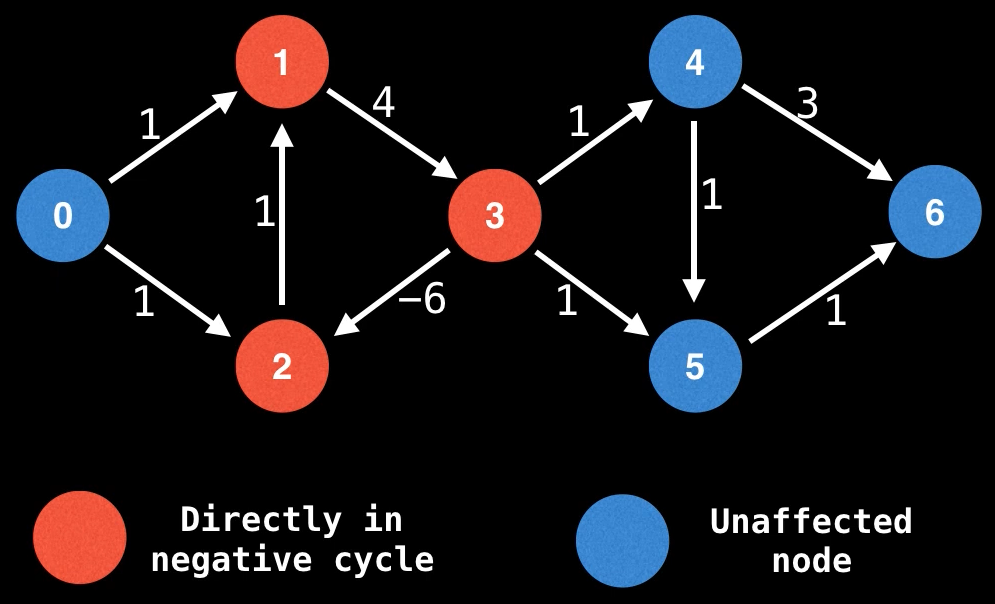
Example shortest path reconstructions

Source	Destination	Shortest Path	Description
`3`	`6`	`None`	Vertex `3` is part of a negative cycle.
`5`	`4`	`[]`	It is impossible to get from vertex `5` to vertex `4`.
`0`	`4`	`None`	The path from `0` to `4` can go through vertices that are part of a negative cycle; thus, the shortest path from `0` to `4` has been compromised.
`4`	`6`	`[4, 5, 6]`	The shortest path from `4` to `6` is `4 -> 5 -> 6` with a total weight of `1 + 1 = 2`.

Output

The final dp table (i.e., APSP solution table) is as follows:

[[0, -inf, -inf, -inf, -inf, -inf, -inf], [inf, -inf, -inf, -inf, -inf, -inf, -inf], [inf, -inf, -inf, -inf, -inf, -inf, -inf], [inf, -inf, -inf, -inf, -inf, -inf, -inf], [inf, inf, inf, inf, 0, 1, 2], [inf, inf, inf, inf, inf, 0, 1], [inf, inf, inf, inf, inf, inf, 0]]

This table can be visualized more effectively in the following way (the entries referenced above regarding shortest path reconstructions are highlighted in red):

$D^6$	$\textcolor{burlywood}{\texttt{0}}$	$\textcolor{burlywood}{\texttt{1}}$	$\textcolor{burlywood}{\texttt{2}}$	$\textcolor{burlywood}{\texttt{3}}$	$\textcolor{burlywood}{\texttt{4}}$	$\textcolor{burlywood}{\texttt{5}}$	$\textcolor{burlywood}{\texttt{6}}$
$\textcolor{burlywood}{\texttt{0}}$	$0$	$-\infty$	$-\infty$	$-\infty$	$\color{red}{-\infty}$	$-\infty$	$-\infty$
$\textcolor{burlywood}{\texttt{1}}$	$\infty$	$-\infty$	$-\infty$	$-\infty$	$-\infty$	$-\infty$	$-\infty$
$\textcolor{burlywood}{\texttt{2}}$	$\infty$	$-\infty$	$-\infty$	$-\infty$	$-\infty$	$-\infty$	$-\infty$
$\textcolor{burlywood}{\texttt{3}}$	$\infty$	$-\infty$	$-\infty$	$-\infty$	$-\infty$	$-\infty$	$\color{red}{-\infty}$
$\textcolor{burlywood}{\texttt{4}}$	$\infty$	$\infty$	$\infty$	$\infty$	$0$	$1$	$\color{red}{2}$
$\textcolor{burlywood}{\texttt{5}}$	$\infty$	$\infty$	$\infty$	$\infty$	$\color{red}{\infty}$	$0$	$1$
$\textcolor{burlywood}{\texttt{6}}$	$\infty$	$\infty$	$\infty$	$\infty$	$\infty$	$\infty$	$0$

Predecessor table

The final pred table (i.e., predecessors table) is as follows:

[[0, -1, -1, -1, -1, -1, -1], [None, -1, -1, -1, -1, -1, -1], [None, -1, -1, -1, -1, -1, -1], [None, -1, -1, -1, -1, -1, -1], [None, None, None, None, 4, 4, 5], [None, None, None, None, None, 5, 5], [None, None, None, None, None, None, 6]]

This can be visualized more effectively in the following way:

$\Pi$	$\textcolor{burlywood}{\texttt{0}}$	$\textcolor{burlywood}{\texttt{1}}$	$\textcolor{burlywood}{\texttt{2}}$	$\textcolor{burlywood}{\texttt{3}}$	$\textcolor{burlywood}{\texttt{4}}$	$\textcolor{burlywood}{\texttt{5}}$	$\textcolor{burlywood}{\texttt{6}}$
$\textcolor{burlywood}{\texttt{0}}$	$0$	$-1$	$-1$	$-1$	$-1$	$-1$	$-1$
$\textcolor{burlywood}{\texttt{1}}$	`None`	$-1$	$-1$	$-1$	$-1$	$-1$	$-1$
$\textcolor{burlywood}{\texttt{2}}$	`None`	$-1$	$-1$	$-1$	$-1$	$-1$	$-1$
$\textcolor{burlywood}{\texttt{3}}$	`None`	$-1$	$-1$	$-1$	$-1$	$-1$	$-1$
$\textcolor{burlywood}{\texttt{4}}$	`None`	`None`	`None`	`None`	$4$	$4_{\color{red}{3}}$	$5_{\color{red}{2}}$
$\textcolor{burlywood}{\texttt{5}}$	`None`	`None`	`None`	`None`	`None`	$5$	$5$
$\textcolor{burlywood}{\texttt{6}}$	`None`	`None`	`None`	`None`	`None`	`None`	$6_{\color{red}{1}}$

Example usage: For the shortest path from 4 to 6, 4 -> 5 -> 6, note how the table above is used to reconstruct this shortest path. Specifically, we start at 6 (the destination vertex), indicated by $6_{\color{red}{1}}$ ; then move to pred[start][curr] = pred[4][6] = 5, indicated by $5_{\color{red}{2}}$ ; then move to pred[start][curr] = pred[4][5] = 4, indicated by $4_{\color{red}{3}}$ . And we're done (we've reached and accounted for the starting vertex). The shortest path has been reconstructed in reverse order: 6 -> 5 -> 4.

Interactive code

The results above may be obtained by running the following code (try it yourself to confirm; modify the code to experiment):

Output

Click "Run Code" to see the output here

Example 3

Graph input (source)

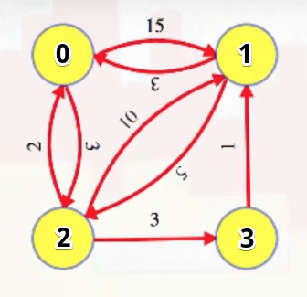
Example shortest path reconstructions

Source	Destination	Shortest Path	Description
`0`	`3`	`[0, 2, 3]`	The shortest path from `0` to `3` is `0 -> 2 -> 3` with a total weight of `3 + 3 = 6`.
`2`	`1`	`[2, 3, 1]`	The shortest path from `2` to `1` is `2 -> 3 -> 1` with a total weight of `3 + 1 = 4`.

Output

The final dp table (i.e., APSP solution table) is as follows:

[[0, 7, 3, 6], [3, 0, 5, 8], [2, 4, 0, 3], [4, 1, 6, 0]]

This table can be visualized more effectively in the following way (the entries referenced above regarding shortest path reconstructions are highlighted in red):

$D^3$	$\textcolor{burlywood}{\texttt{0}}$	$\textcolor{burlywood}{\texttt{1}}$	$\textcolor{burlywood}{\texttt{2}}$	$\textcolor{burlywood}{\texttt{3}}$
$\textcolor{burlywood}{\texttt{0}}$	$0$	$7$	$3$	$\color{red}{6}$
$\textcolor{burlywood}{\texttt{1}}$	$3$	$0$	$5$	$8$
$\textcolor{burlywood}{\texttt{2}}$	$2$	$\color{red}{4}$	$0$	$3$
$\textcolor{burlywood}{\texttt{3}}$	$4$	$1$	$6$	$0$

Predecessor table

The final pred table (i.e., predecessors table) is as follows:

[[0, 3, 0, 2], [1, 1, 1, 2], [2, 3, 2, 2], [1, 3, 1, 3]]

This can be visualized more effectively as follows:

$\Pi$	$\textcolor{burlywood}{\texttt{0}}$	$\textcolor{burlywood}{\texttt{1}}$	$\textcolor{burlywood}{\texttt{2}}$	$\textcolor{burlywood}{\texttt{3}}$
$\textcolor{burlywood}{\texttt{0}}$	$0$	$3$	$0$	$2$
$\textcolor{burlywood}{\texttt{1}}$	$1$	$1_{\color{red}{1}}$	$1$	$2$
$\textcolor{burlywood}{\texttt{2}}$	$2$	$3_{\color{red}{2}}$	$2$	$2_{\color{red}{3}}$
$\textcolor{burlywood}{\texttt{3}}$	$1$	$3$	$1$	$3$

Example usage: For the shortest path from 2 to 1, 2 -> 3 -> 1, note how the table above is used to reconstruct this shortest path. Specifically, we start at 1 (the destination vertex), indicated by $1_{\color{red}{1}}$ ; then move to pred[start][curr] = pred[2][1] = 3, indicated by $3_{\color{red}{2}}$ ; then move to pred[start][curr] = pred[2][3] = 2, indicated by $2_{\color{red}{3}}$ . And we're done (we've reached and accounted for the starting vertex). The shortest path has been reconstructed in reverse order: 1 -> 3 -> 2.

Interactive code

The results above may be obtained by running the following code (try it yourself to confirm; modify the code to experiment):

Output

Click "Run Code" to see the output here

Example 4

Graph input (source)

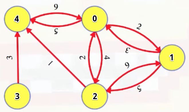
Example shortest path reconstructions

Source	Destination	Shortest Path	Description
`2`	`3`	`[]`	It is impossible to get from vertex `2` to vertex `3`.
`3`	`1`	`[3, 4, 0, 1]`	The shortest path from `3` to `1` is `3 -> 4 -> 0 -> 1` with a total weight of `3 + 9 + 2 = 14`.

Output

The final dp table (i.e., APSP solution table) is as follows:

[[0, 2, 4, inf, 5], [3, 0, 5, inf, 6], [2, 4, 0, inf, 1], [12, 14, 16, 0, 3], [9, 11, 13, inf, 0]]

This table can be visualized more effectively in the following way (the entries referenced above regarding shortest path reconstructions are highlighted in red):

$D^4$	$\textcolor{burlywood}{\texttt{0}}$	$\textcolor{burlywood}{\texttt{1}}$	$\textcolor{burlywood}{\texttt{2}}$	$\textcolor{burlywood}{\texttt{3}}$	$\textcolor{burlywood}{\texttt{4}}$
$\textcolor{burlywood}{\texttt{0}}$	$0$	$2$	$4$	$\infty$	$5$
$\textcolor{burlywood}{\texttt{1}}$	$3$	$0$	$5$	$\infty$	$6$
$\textcolor{burlywood}{\texttt{2}}$	$2$	$4$	$0$	$\color{red}{\infty}$	$1$
$\textcolor{burlywood}{\texttt{3}}$	$12$	$\color{red}{14}$	$16$	$0$	$3$
$\textcolor{burlywood}{\texttt{4}}$	$9$	$11$	$13$	$\infty$	$0$

Predecessor table

The final pred table (i.e., predecessors table) is as follows:

[[0, 0, 0, None, 0], [1, 1, 1, None, 2], [2, 0, 2, None, 2], [4, 0, 0, 3, 3], [4, 0, 0, None, 4]]

This can be visualized more effectively as follows:

$\Pi$	$\textcolor{burlywood}{\texttt{0}}$	$\textcolor{burlywood}{\texttt{1}}$	$\textcolor{burlywood}{\texttt{2}}$	$\textcolor{burlywood}{\texttt{3}}$	$\textcolor{burlywood}{\texttt{4}}$
$\textcolor{burlywood}{\texttt{0}}$	$0$	$0$	$0$	`None`	$0$
$\textcolor{burlywood}{\texttt{1}}$	$1$	$1_{\color{red}{1}}$	$1$	`None`	$2$
$\textcolor{burlywood}{\texttt{2}}$	$2$	$0$	$2$	`None`	$2$
$\textcolor{burlywood}{\texttt{3}}$	$4_{\color{red}{3}}$	$0_{\color{red}{2}}$	$0$	$3$	$3_{\color{red}{4}}$
$\textcolor{burlywood}{\texttt{4}}$	$4$	$0$	$0$	`None`	$4$

Example usage: For the shortest path from 3 to 1, 3 -> 4 -> 0 -> 1, note how the table above is used to reconstruct this shortest path. Specifically, we start at 1 (the destination vertex), indicated by $1_{\color{red}{1}}$ ; then move to pred[start][curr] = pred[3][1] = 0, indicated by $0_{\color{red}{2}}$ ; then move to pred[start][curr] = pred[3][0] = 4, indicated by $4_{\color{red}{3}}$ ; then move to pred[start][curr] = pred[3][4] = 3, indicated by $3_{\color{red}{4}}$ . And we're done (we've reached and accounted for the starting vertex). The shortest path has been reconstructed in reverse order: 1 -> 0 -> 4 -> 3.

Interactive code

The results above may be obtained by running the following code (try it yourself to confirm; modify the code to experiment):

Output

Click "Run Code" to see the output here

Example 5

Graph input (source)

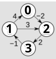
Example shortest path reconstructions

Source	Destination	Shortest Path	Description
`1`	`2`	`[1, 0, 2]`	The shortest path from `1` to `2` is `1 -> 0 -> 2` with a total weight of `4 + (-2) = 2`.
`3`	`2`	`[3, 1, 0, 2]`	The shortest path from `3` to `2` is `3 -> 1 -> 0 -> 2` with a total weight of `(-1) + 4 + (-2) = 1`.

Output

The final dp table (i.e., APSP solution table) is as follows:

[[0, -1, -2, 0], [4, 0, 2, 4], [5, 1, 0, 2], [3, -1, 1, 0]]

This table can be visualized more effectively in the following way (the entries referenced above regarding shortest path reconstructions are highlighted in red):

$D^3$	$\textcolor{burlywood}{\texttt{0}}$	$\textcolor{burlywood}{\texttt{1}}$	$\textcolor{burlywood}{\texttt{2}}$	$\textcolor{burlywood}{\texttt{3}}$
$\textcolor{burlywood}{\texttt{0}}$	$0$	$-1$	$-2$	$0$
$\textcolor{burlywood}{\texttt{1}}$	$4$	$0$	$\color{red}{2}$	$4$
$\textcolor{burlywood}{\texttt{2}}$	$5$	$1$	$0$	$2$
$\textcolor{burlywood}{\texttt{3}}$	$3$	$-1$	$\color{red}{1}$	$0$

Predecessor table

The final pred table (i.e., predecessors table) is as follows:

[[0, 3, 0, 2], [1, 1, 0, 2], [1, 3, 2, 2], [1, 3, 0, 3]]

This can be visualized more effectively as follows:

$\Pi$	$\textcolor{burlywood}{\texttt{0}}$	$\textcolor{burlywood}{\texttt{1}}$	$\textcolor{burlywood}{\texttt{2}}$	$\textcolor{burlywood}{\texttt{3}}$
$\textcolor{burlywood}{\texttt{0}}$	$0$	$3$	$0$	$2$
$\textcolor{burlywood}{\texttt{1}}$	$1$	$1$	$0$	$2$
$\textcolor{burlywood}{\texttt{2}}$	$1$	$3$	$2_{\color{red}{1}}$	$2$
$\textcolor{burlywood}{\texttt{3}}$	$1_{\color{red}{3}}$	$3_{\color{red}{4}}$	$0_{\color{red}{2}}$	$3$

Example usage: For the shortest path from 3 to 2, 3 -> 1 -> 0 -> 2, note how the table above is used to reconstruct this shortest path. Specifically, we start at 2 (the destination vertex), indicated by $2_{\color{red}{1}}$ ; then move to pred[start][curr] = pred[3][2] = 0, indicated by $0_{\color{red}{2}}$ ; then move to pred[start][curr] = pred[3][0] = 1, indicated by $1_{\color{red}{3}}$ ; then move to pred[start][curr] = pred[3][1] = 3, indicated by $3_{\color{red}{4}}$ . And we're done (we've reached and accounted for the starting vertex). The shortest path has been reconstructed in reverse order: 2 -> 0 -> 1 -> 3.

Interactive code

The results above may be obtained by running the following code (try it yourself to confirm; modify the code to experiment):

Output

Click "Run Code" to see the output here

Example 6

Graph input (source: [21])

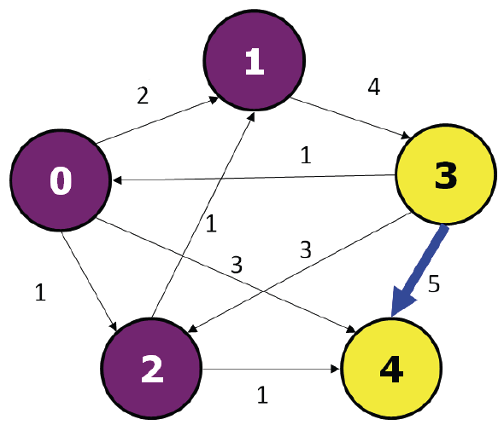
Example shortest path reconstructions

Source	Destination	Shortest Path	Description
`4`	`2`	`[]`	It is impossible to get from vertex `4` to vertex `2`.
`3`	`4`	`[3, 0, 2, 4]`	The shortest path from `3` to `4` is `3 -> 0 -> 2 -> 4` with a total weight of `1 + 1 + 1 = 3`.
`1`	`4`	`[1, 3, 0, 2, 4]`	The shortest path from `3` to `1` is `1 -> 3 -> 0 -> 2 -> 4` with a total weight of `4 + 1 + 1 + 1 = 7`.

Output

The final dp table (i.e., APSP solution table) is as follows:

[[0, 2, 1, 6, 2], [5, 0, 6, 4, 7], [6, 1, 0, 5, 1], [1, 3, 2, 0, 3], [inf, inf, inf, inf, 0]]

This table can be visualized more effectively in the following way (the entries referenced above regarding shortest path reconstructions are highlighted in red):

$D^4$	$\textcolor{burlywood}{\texttt{0}}$	$\textcolor{burlywood}{\texttt{1}}$	$\textcolor{burlywood}{\texttt{2}}$	$\textcolor{burlywood}{\texttt{3}}$	$\textcolor{burlywood}{\texttt{4}}$
$\textcolor{burlywood}{\texttt{0}}$	$0$	$2$	$1$	$6$	$2$
$\textcolor{burlywood}{\texttt{1}}$	$5$	$0$	$6$	$4$	$\color{red}{7}$
$\textcolor{burlywood}{\texttt{2}}$	$6$	$1$	$0$	$5$	$1$
$\textcolor{burlywood}{\texttt{3}}$	$1$	$3$	$2$	$0$	$\color{red}{3}$
$\textcolor{burlywood}{\texttt{4}}$	$\infty$	$\infty$	$\color{red}{\infty}$	$\infty$	$0$

Predecessor table

The final pred table (i.e., predecessors table) is as follows:

[[0, 0, 0, 1, 2], [3, 1, 0, 1, 2], [3, 2, 2, 1, 2], [3, 0, 0, 3, 2], [None, None, None, None, 4]]

This can be visualized more effectively as follows:

$\Pi$	$\textcolor{burlywood}{\texttt{0}}$	$\textcolor{burlywood}{\texttt{1}}$	$\textcolor{burlywood}{\texttt{2}}$	$\textcolor{burlywood}{\texttt{3}}$	$\textcolor{burlywood}{\texttt{4}}$
$\textcolor{burlywood}{\texttt{0}}$	$0$	$0$	$0$	$1$	$2$
$\textcolor{burlywood}{\texttt{1}}$	$3_{\color{red}{4}}$	$1$	$0_{\color{red}{3}}$	$1_{\color{red}{5}}$	$2_{\color{red}{2}}$
$\textcolor{burlywood}{\texttt{2}}$	$3$	$2$	$2$	$1$	$2$
$\textcolor{burlywood}{\texttt{3}}$	$3$	$0$	$0$	$3$	$2$
$\textcolor{burlywood}{\texttt{4}}$	`None`	`None`	`None`	`None`	$4_{\color{red}{1}}$

Example usage: For the shortest path from 1 to 4, 1 -> 3 -> 0 -> 2 -> 4, note how the table above is used to reconstruct this shortest path. Specifically, we start at 4 (the destination vertex), indicated by $4_{\color{red}{1}}$ ; then move to pred[start][curr] = pred[1][4] = 2, indicated by $2_{\color{red}{2}}$ ; then move to pred[start][curr] = pred[1][2] = 0, indicated by $0_{\color{red}{3}}$ ; then move to pred[start][curr] = pred[1][0] = 3, indicated by $3_{\color{red}{4}}$ ; then move to pred[start][curr] = pred[1][3] = 1, indicated by $1_{\color{red}{5}}$ . And we're done (we've reached and accounted for the starting vertex). The shortest path has been reconstructed in reverse order: 4 -> 2 -> 0 -> 3 -> 1.

Interactive code

The results above may be obtained by running the following code (try it yourself to confirm; modify the code to experiment):

Output

Click "Run Code" to see the output here

Introduction to dynamic programming - Fibonacci numbers​

Fibonacci number definition​

Simple recursive algorithm​

Recursion tree​

Memoized algorithm​

Pruned recursion tree​

Alternate version (order of recursively computed values)​

Table fill order​

Iterating to eliminate recursion​

Optimizing space​

Modular indexing​

Variable assignment​

Additional example - Tribonacci numbers​

Dynamic programming template​

The rod cutting problem​

Problem definition​

Dynamic programming template​

Recursive solution design​

Recursive solution​

Recursive tree​

Parameter analysis​

Memoized top-down DP approach​

Memoized recursive tree​

Tabulated bottom-up DP approach​

Reconstructing the optimal cuts​

The subset sum problem​

Problem definition​

Dynamic programming outline​

Recursive idea 1​

Recursive algorithm​

Parameter problems​

Recursive idea 2​

Recursive algorithm​

Memoized version​

Iterative version​

Space optimization​

Reconstructing the set?​

Recursive idea 3​

Memoized version​

Iterative version​

Space optimization​

Reconstructing the set​

Analysis​

Floyd-Warshall​

Template (TLDR)​

William Fiset presentation of Floyd-Warshall​

Algorithm overview​

SP algorithms​

Graph setup​

Main concept​

The memo table​

Floyd-Warshall algorithm​

Pseudocode​

Pseudocode discussion​

Steven Halim presentation of Floyd-Warshall​

Algorithms with Attitude presentation of Floyd-Warshall​

Problem definition​

Recursive idea​

Recursive algorithm​

Memoization​

Iterative version​

Space optimization​

Origin story​

Reconstructing paths​

Interactive examples​

Example 1​

Graph input (source)​

Example shortest path reconstructions​

Output​

Predecessor table​

Interactive code​

Example 2​

Graph input (source)​

Example shortest path reconstructions​

Output​

Predecessor table​

Interactive code​

Example 3​

Graph input (source)​

Example shortest path reconstructions​

Introduction to dynamic programming - Fibonacci numbers

Fibonacci number definition

Simple recursive algorithm

Recursion tree

Memoized algorithm

Pruned recursion tree

Alternate version (order of recursively computed values)

Table fill order

Iterating to eliminate recursion

Optimizing space

Modular indexing

Variable assignment

Additional example - Tribonacci numbers

Dynamic programming template

The rod cutting problem

Problem definition

Dynamic programming template

Recursive solution design

Recursive solution

Recursive tree

Parameter analysis

Memoized top-down DP approach

Memoized recursive tree

Tabulated bottom-up DP approach

Reconstructing the optimal cuts

The subset sum problem

Problem definition

Dynamic programming outline

Recursive idea 1

Recursive algorithm

Parameter problems

Recursive idea 2

Recursive algorithm

Memoized version

Iterative version

Space optimization

Reconstructing the set?

Recursive idea 3

Memoized version

Iterative version

Space optimization

Reconstructing the set

Analysis

Floyd-Warshall

Template (TLDR)

William Fiset presentation of Floyd-Warshall

Algorithm overview

SP algorithms

Graph setup

Main concept

The memo table

Floyd-Warshall algorithm

Pseudocode

Pseudocode discussion

Steven Halim presentation of Floyd-Warshall

Algorithms with Attitude presentation of Floyd-Warshall

Problem definition

Recursive idea

Recursive algorithm

Memoization

Iterative version

Space optimization

Origin story

Reconstructing paths

Interactive examples

Example 1

Graph input (source)

Example shortest path reconstructions

Output

Predecessor table

Interactive code

Example 2

Graph input (source)

Example shortest path reconstructions

Output

Predecessor table

Interactive code

Example 3

Graph input (source)

Example shortest path reconstructions