Learning Tarjan's algorithm

Learning Tarjan's algorithm for finding the strongly connected components (SCCs) of a directed graph can be rather difficult at first. Many learning materials sketch out the concepts and may even provide pseudocode, but few materials provide fully worked out examples along with working code. This blog post seeks to change that. Example graphs are taken from other quality learning sources (with attribution), but, importantly, working code is provided (in Python) to test Tarjan's algorithm to see the results for yourself.

TLDR

The following code may be used as a template for implementing Tarjan's algorithm. The input is assumed to be an adjacency list of index arrays, and the output is a list of the strongly connected components for the input graph in reverse topological order.

Tarjan's algorithm (Python implementation)

# T: O(V + E); S: O(V)
def tarjan(graph):
    n = len(graph)          # graph assumed to be adjacency list of index arrays
    node_id = 0             # unique node_id assigned to each node
    ids = [-1] * n          # id of each node
    low_link = [0] * n      # store lowest id node reachable from each node
    on_stack = [False] * n  # boolean array to check if a node is on the stack
    stack = []              # stack to keep track of nodes in current SCC
    sccs = []               # list to store all SCCs

    def dfs(node):
        nonlocal node_id
        low_link[node] = node_id    # initialize low_link value of node to be its own node_id
        ids[node] = node_id         # assign smallest unused node_id to node
        node_id += 1                # increment node_id value to ensure later nodes have higher node_id values
        stack.append(node)          # push node onto the stack
        on_stack[node] = True       # mark node as being on the stack

        # explore all outgoing edges from the node
        for nbr in graph[node]:
            if ids[nbr] == -1:      # visit nbr if it has not yet been visited
                dfs(nbr)
            if on_stack[nbr]:       # nbr is on stack, thus part of current SCC (minimize low-link on callback)
                low_link[node] = min(low_link[node], low_link[nbr])

        # if node is a root node of an SCC, pop from stack and generate SCC
        if ids[node] == low_link[node]:
            scc = []
            while stack:
                scc_nbr = stack.pop()
                on_stack[scc_nbr] = False
                low_link[scc_nbr] = ids[node]
                scc.append(scc_nbr)
                if scc_nbr == node:
                    break
                
            sccs.append(scc)  # add SCC to overall list of SCCs

    # initialize top-level DFS traversals
    for v in range(n):
        if ids[v] == -1:
            dfs(v)

    return sccs  # return list of SCCs

Building intuition for Tarjan's algorithm

Attribution

What follows in this section is largely the written form of William Fiset's excellent video on Tarjan's algorithm. But the linked video

What SCCs actually are

It helps if we first ask ourselves what strongly connected components (SCCs) actually are. The following is a suitable working definition:

Strongly connected components (SCCs) can be thought of as self-contained cycles within a directed graph where every vertex in a given cycle can reach every other vertex in the same cycle.

Consider the following graph as an example (original graph on the left and its SCCs highlight and isolated on the right):

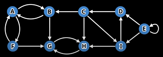
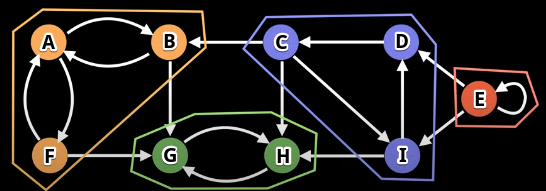
If we inspect each SCC above, then we will see that each SCC has its own self-contained cycle, and, for each SCC, there is no way to find a path that leaves a component and comes back. Because of this property, we can be certain that SCCs in a graph are unique.

The component graph and topological orderings

What other consequences may there be due to a path leaving a component but not being able to come back?

Suppose we somehow know in advance what the SCCs are for a graph. Further suppose we "collapse" the graph down into different "super-vertices", where each vertex represents a component. In the previously pictured graph, we could imagine the following as super-vertices (each vertex label represents the underlying members, in no particular order, of the SCC it represents): ABF, GH, CDI, and E.

How are the super-vertices above connected to each other? We have the following "edges" between super-vertices:

• ABF: ABF -> GH
• GH: No outgoing edges
• CDI: CDI -> GH, CDI -> ABF
• E: E -> E, E -> CDI

The edges above comprise the so-called component graph whose vertices are the super-vertices (SCCs) and the edges are as detailed above.

The observation directly above this note, specifically that there is no way to find a path that leaves a component and comes back, provides a neat clue as to the underlying structure of the component graph and the ultimate result returned by Tarjan's algorithm.

Specifically, the component graph represented with the super-vertices and edges above lead to the following topological order of the super-vertices:

Tarjan's algorithm ultimately returns the reverse of the topological ordering above (i.e., a reverse topological sort of a graph's super-vertices or SCCs).

What about self-loops?

Note that the topological sort shown above does not picture the original self-loop for vertex E. Why? Isn't it true that a graph must be directed and acyclic in order for a topological ordering to exist? Yes. So how can we get by with just deleting the self-loop?

The answer lies in what we care about cycles being between.

• General directed graphs (vertices): For general graphs, a self-loop is considered a cycle and prevents the existence of a topological ordering. We care about cycles existing between vertices (even if a single vertex serves as both endpoints for an edge, which is the case with a self-loop). If a graph had a vertex X that induced a self-loop, then X would have itself as a dependency (in the language of topological sorts), meaning that X can never be resolved. Hence, a general graph must be directed and acyclic (DAG) in order for a topological ordering of its vertices to exist. Self-loops are disqualifying.
• Component graphs (strongly connected components): For component graphs, SCCs are collapsed into single nodes or "super-vertices". Importantly, self-loops within SCCs are absorbed into these super-vertices. Why? Because the component graph represents cycles between SCCs; that is, self-loops indicate internal cycles within an SCC but does not create cycles between different SCCs. This is normal and to be expected; indeed, an SCC is a cycle by definition — simply having another vertex (or several) with a self-loop as part of the cycle does not change anything.

Essentially, the key observation is that the component graph is acyclic between SCCs, which means the SCCs can be topologically ordered (even if self-loops exist within them).

We can reference a more offical source such as [21] for more complete information. Specifically, strongly connected components are defined as follows in [21]:

The strongly connected components of a directed graph are the equivalence classes of vertices under the "are mutually reachable" relation.

Concerning equivalence classes under the "mutually reachable" relation, this just means the following:

• Reflexivity: A vertex can reach itself either by not moving at all or having a self-loop
• Symmetry: If vertex A can reach vertex B, then vertex B can reach vertex A (symmetry)
• Transitivity: If vertex A can reach vertex B and vertex B can reach vertex C, then vertex A can reach vertex C.

The graph below is provided as an example:

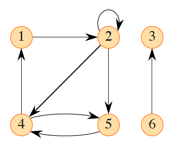
The following justification is given:

There are three strongly connected components: $\{1,2,4,5\}$, $\{3\}$, and $\{6\}$. All pairs of vertices in $\{1,2,4,5\}$ are mutually reachable. The vertices $\{3,6\}$ do not form a strongly connected component, since vertex 6 cannot be reached from vertex 3.

Another more detailed example involving strongly connected components may be found in [21] (disregard numbers within the vertices that represent DFS discovery and finish times; note how the original graph on the left, where SCCs are highlighted in blue, is collapsed into the component graph on the right):

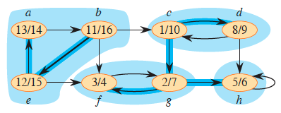
The acyclic component graph (right) is obtained by contracting all edges within each SCC so that only a single vertex remains in each component. Specifically, note how vertex h is its own SCC and has a self-loop.

The gist: self-loops do not cause problems when we're trying to find SCCs because the acyclicity we care about is between SCCs (not individual vertices, as we might be for general graphs). CLRS goes on to state a lemma that "gives the key property that the component graph is acyclic." Many more details may be found within that text.

Low-link values

To understand Tarjan's algorithm, we're first going to need to understand the concept of a low-link value:

The low-link value of a node is the smallest (lowest) node id reachable from that node (including the id of the node itself) when doing a DFS.

For the definition above to make sense, let's first label the vertices of the graph on the left, starting from 0, by doing a DFS. One possible result is the graph on the right (depending on the order in which neighbors are visited):

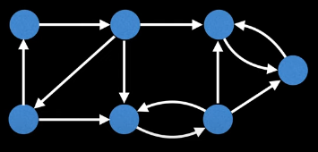
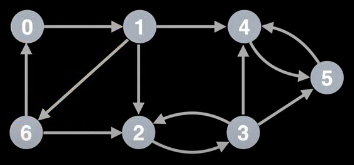
Now let's try to inspect the graph to determine the low-link value of each node. Doing so yields the following:

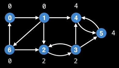
The rationale behind each calculation is summarized in the following table:

Node	Low-link value	Reason
0	0	The smallest node id is the id of the node itself, namely 0.
1	0	Node 0 can be reached from node 1: 1 -> 6 -> 0.
2	2	Node 2 cannot reach node 0 or node 1; hence, the smallest id is its own id, 2.
3	2	Node 3 can reach node 2 but not any node with a smaller id: 3 -> 2.
4	4	Only node 5 can be reached from node 4, but 5 is a bigger id that 4.
5	4	The only smaller id node that node 5 can reach is node 4: 5 -> 4
6	0	Node 0 can be reached from node 6: 6 -> 0

The view of the graph above, where low-link values are shown beside their nodes, shows that all nodes having the same low-link value belong to the same SCC:

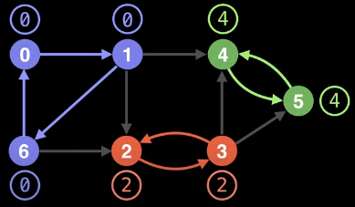
If what's been shown so far is all that's involved in finding the SCCs for a directed graph, then it doesn't seem like it should be all that difficult. What's the catch? The catch with the "technique" shown above is that it is highly dependent on the traversal order of the DFS, which is essentially random. What happens if we start the DFS from a different node?

For example:

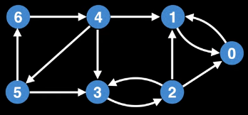
The graph above is the exact same as the graph we had previously, but this time nodes ids are shifted around. This time, we're going to start our DFS at the node on the far right. It gets id 0. The top-level DFS call to each node would look as follows:

• Node 0: This is where we start. We discover only one other node from this search, namely the node to which we gave the label 1.
• Node 1: We already discovered this node so we move on.
• Node 2: We discover only one more node in this search and give it label 3.
• Node 3: We already discovered this node so we move on.
• Node 4: We skip over nodes 1 and 3 since they've already been visited, but we discover node 5, and continuing our search from node 5 leads us to discover the last node, which we give label 6.
• We do not conduct a DFS on nodes 5 and 6 since they've already been discovered.

What are the low-link values for each node now (with the new DFS traversal order)? It's 0 for every single node!

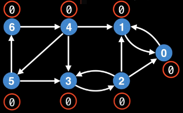
This is a problem. All low-link values are the same, but there are clearly multiple SCCs. What's going on? What's happening is that the low-link values are highly dependent on the order in which nodes are explored during the DFS. Hence, we might not end up with a correct arrangement of node ids for our low-link values to tell us which nodes are in which SCCs.

This important lesson bears repeating: Depending on where the DFS starts, and the order in which nodes/edges are visited, the low-link values for identifying SCCs could be wrong.

What are we to do? If we still want to use low-link values to identify SCCs somehow, then we need to come up with a way to ensure the low-link values of nodes in one SCC do not interfere with the low-link values of nodes in another SCC. This is where Tarjan's algorithm comes into play. Robert Tarjan came up with a clever way to do this by strategically using a stack invariant: the stack invariant is used to prevent low-link values of multiple SCCs from interfering with each other.

To cope with the random traversal order of the DFS, Tarjan's algorithm maintains a set (often implemented as a stack) of valid nodes from which to update low-link values from. Nodes are pushed to the stack of valid nodes as they're explored for the first time, and nodes are popped from the stack each time a complete SCC is found.

The statements above will make more sense if we first consider a new condition for updating low-link values and then contextualize the new update by means of a fully worked example. If u and v are nodes in a graph and we're currently exploring u, then our new low-link update condition is as follows: To update node u's low-link value to node v's low-link value, there has to be a path of edges from u to v, and node v must be on the stack.

To optimize for time efficiency, we're not going to find all low-link values after the fact (i.e., doing a DFS for each node and then finding low-link values); instead, we're going to update low-link values "on the fly" during the DFS in order to get a linear $O(V + E)$ time complexity. This will make this algorithm very efficient.

High-level overview of Tarjan's algorithm

Before analyzing a fully worked example, here's a high-level overview of Tarjan's algorithm to contextualize the mechanics a bit more:

• Mark the id of each node as unvisited.
• Start DFS (from any node). Upon visiting a node, assign it an id and a low-link value equal to that id. Increment the id for subsequent node id assignments. Also mark current nodes as visited and add them to a seen stack.
• On DFS callback (i.e., after the recursion comes back once the search hits a dead end and we need to backtrack), if the node we are backtracking from is on the stack, then take the minimum of the current node's low-link value with the low-link value of the node we are backtracking from (this allows low-link values to propagate throughout cycles).
• After visiting all neighbors, if the current node started a connected component, then pop nodes off the stack until the current node is reached. (As we will see, a node started a connected component if its id equals its low-link value.)

Fully worked example

Reference the pseudocode and Python implementation (as needed)

Throughout the course of the fully worked example, it may help at different moments to consult either the pseudocode or the implementation (or both).

Everything above will make more sense after we've worked through a detailed example. To that end, consider the following graph:

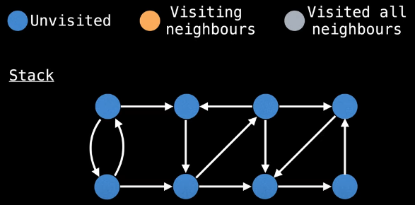
If a node's color is grey or orange, then it is on the stack, and we can update its low-link value per the low-link update condition mentioned previously:

To update node u's low-link value to node v's low-link value, there has to be a path of edges from u to v, and node v must be on the stack.

The nodes on the stack will be tracked in the left column beside the pictured graph (under the "Stack" heading). Let's start our DFS in a truly random fashion: bottom row, second node from right:

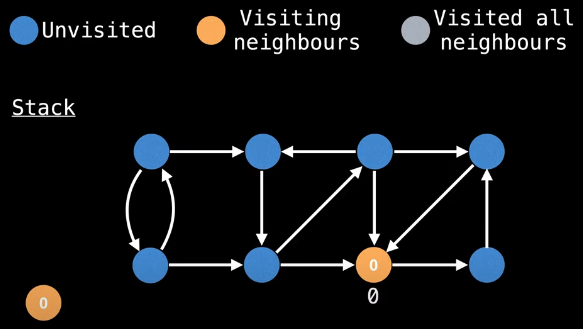
As we explore unvisited nodes, give each node an id and a low-link value equal to that id. If we start our DFS as illustrated above, then once we reach node 2, our only option will then be to visit node 0:

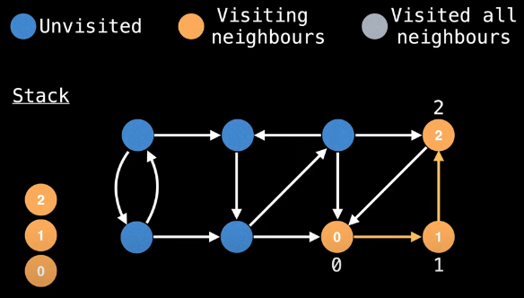
Since node 0 has already been visited, we do not want to visit it again. We're now at the "DFS callback" stage mentioned in the previous section, where we need to start backtracking in order for the recursion to "unwind" — this is where we get to start updating low-link values in a meaningful way. But how exactly?

Once node 2 has been marked as visited, we're still tasked with determining whether or not any of its neighbors have been visited (line 21 of the implementation). We attempt to visit node 0, but we notice it has already been visited; hence, we do not continue the DFS on node 0 (line 22 of the implementation). But is node 0 on the stack (line 23 of the implementation)? Yes, it is; hence, we should update the low-link value of node 2 to be the minimum of the low-link value that currently exists for node 2 as well as the low-link value for the node we were just trying to visit but needed to backtrack from, namely node 0:

low_link[2] = min(low_link[2], low_link[0])
            = 0

We update the visual accordingly:

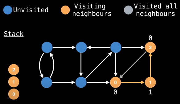
Similarly, once we've gone back to node 2 from node 0 that couldn't be visited again, we see that we need to backtrack from node 2 to node 1:

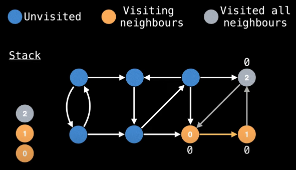
Node 2 is on the stack so we make the appropriate low-link value update:

low_link[1] = min(low_link[1], low_link[2])
            = 0

Now the same goes for needing to backtrack from node 1 to node 0:

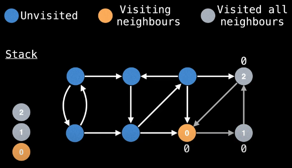
We update the low-link value of node 0 accordingly:

low_link[0] = min(low_link[0], low_link[1])
            = 0

Once we've returned to node 0 and updated its low-link value, we realize that we've actually finished an SCC since the current node has visited all of its neighbors and its low-link value equals its id (line 27 of the implementation):

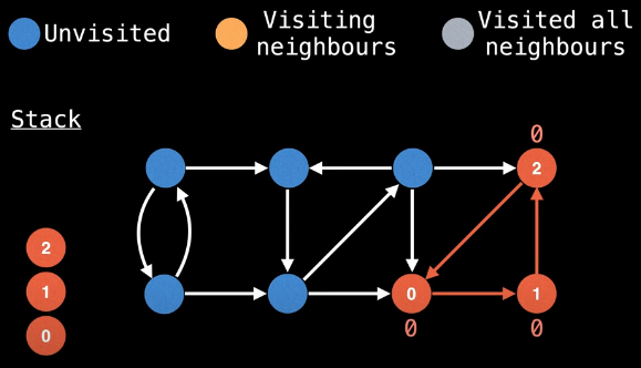
We now need to pop off all associated nodes that are currently on the stack (lines 28-37 of the implementation):

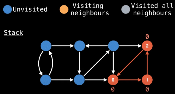
But, of course, we're not yet done exploring the graph. Thus, we pick another node to start a DFS from that has not yet been visited. We'll start at the top left node this time:

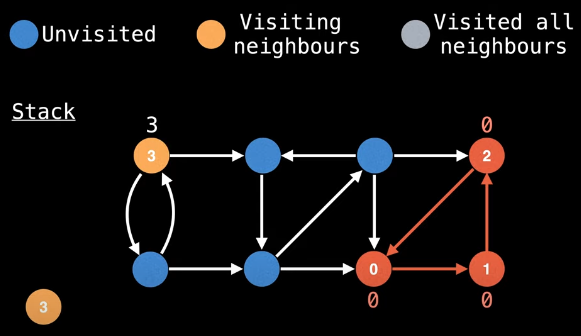
Assigning unique (incremented) node ids, we randomly choose to go right. Then the only direction is to go down. And then we randomly choose to go to the right (instead of diagonally):

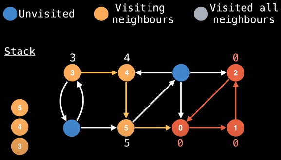
Now, when we try to visit node 0 from node 5, we see that node 0 has already been visited; hence, we need to backtrack from node 0 to node 5 and continue the search. But, during this callback, we first need to see if the low-link value for 5 should be updated. What node did we just backtrack from? Node 0. Is node 0 on the stack? No. So we do not try to update the low-link value for node 5. This is very good because if we tried to update the low-link value for node 5, then we would essentially contaminate the SCC that node 5 is part of with a lower low-link value which node 0 has to offer.

How the stack invariant works and pays off is becoming clearer. Specifically, node 0 not being on the stack is not just a happy coincidence — if node 0 were on the stack, then this would mean there's not only a way to get from node 5 to node 0 but also a way to get from node 0 to node 5, which there isn't.

Since we can't go right to node 0 from node 5 and can't update node 5's low-link value since node 0 is not on the stack, we continue our search diagonally, now to node 6:

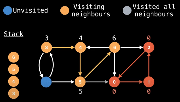
Which direction should we go from node 6? We've already visited nodes 4 (left), 2 (right), and 0 (down). Each choice will result in a callback or need to backtrack to node 6. Suppose we try to visit the neighbors of node 6 by going right, then left, and then down:

• right: node 2 has already been visited and is not on the stack; hence, we cannot update the low-link value for node 6
• left: node 4 has already been visited and is on the stack; hence, we update the low-link value for node 6: low_link[6] = min(low_link[6], low_link[4])
• down: node 0 has already been visited and is not on the stack; hence we cannot update the low-link value for node 6

After attempting the visits above and making the appropriate low-link value update, our visual is as follows:

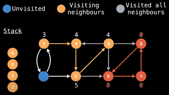
Remember that we started the current DFS on node 3. We have a good bit of backtracking still left to do. Next up, we backtrack from node 6 to node 5. Since node 6 is on the stack, we can update node 5's low-link value:

low_link[5] = min(low_link[5], low_link[6])

Making this update yields the following visual:

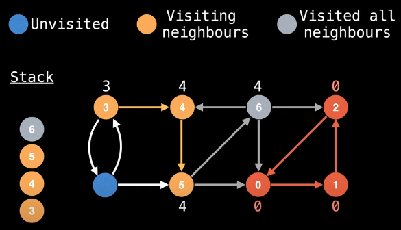
We now backtrack from node 5 to node 4. Since node 5 is on the stack, we can update node 4's low-link value:

low_link[4] = min(low_link[4], low_link[5])

Our visual can now be updated again:

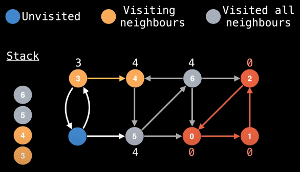
Importantly, we observe that node 4's low-link value and its id are the same, which means we've completed another SCC:

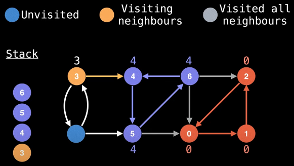
Now we just need to pop the associated nodes from the stack (i.e., 6, 5, and 4, in that order)

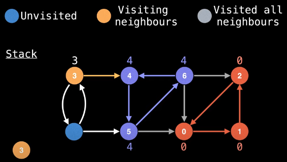
The stack invariant now pays off yet again: backtracking from node 4 to node 3 means we need to see if we can update node 3's low-link value. But 4 is no longer on the stack, which means we can't. Again, this is very good!

Now we're back at node 3, a node whose id is equal to its low-link value. Hence, it may seem as if node 3 should be the start of an SCC. But is it? We cannot make that assessment just yet. Why? Because we have not yet finished visiting all of node 3's neighbors. The check for the start of an SCC (line 27 of the implementation) does not happen until after all neighbors have been visited (lines 20-24 of the implementation) for the top-level DFS (line 11 of the implementation). Hence, even though we started a top-level DFS from node 3 and discovered an SCC along the way in nodes 4, 5, and 6, this does not necessarily mean that node 3 starts its own SCC. We need to visit all of its neighbors first in order to effectively make this assessment.

We now take the downward edge from node 3 to what is now node 7:

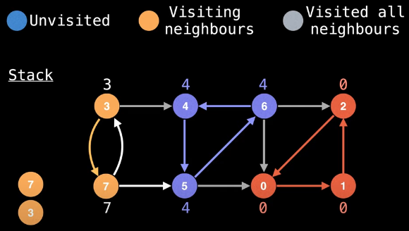
From node 7 we can either go up (back to node 3) or to the right (to node 5). Let's go right:

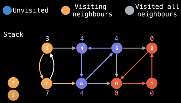
Since node 5 has already been visited, we need to backtrack to node 7. Should we update the low-link value for node 7? No, because node 5 is not on the stack (again, this is very good). Finally, we take the upward edge from node 7 to node 3. But node 3 has already been visited, which means we need to backtrack again to node 7:

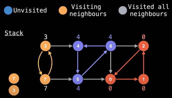
When we backtrack from node 3 to node 7, we see that node 3 is on the stack; hence, we should update node 7's low-link value:

low_link[7] = min(low_link[7], low_link[3])
            = 3

This gives us the following visual:

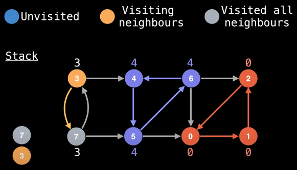
Finally, we need to backtrack from node 7 to node 3. Since node 7 is on the stack, we should update the low-link value for node 3:

low_link[3] = min(low_link[3], low_link[7])
            = 3

Now, at this point, we are back at node 3, we've visited all of node 3's neighbors, and node 3's id is the same as its low-link value:

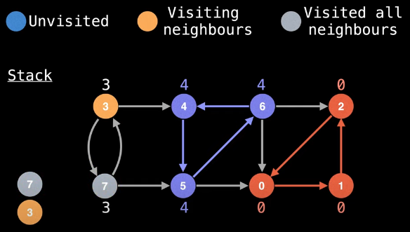
This means node 3 is, in fact, the start of an SCC:

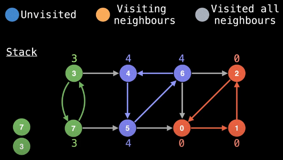
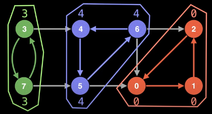
All that remains now is to remove all associated nodes from the stack. Every vertex in the graph has now been discovered and the stack is empty, thus concluding the algorithm which yields all of the SCCs in the graph:

Pseudocode

The pseudocode that follows is taken directly from William Fiset's video linked at the beginning of this post. Descriptions of different lines are provided after the pseudocode.

Pseudocode for Tarjan's algorithm

UNVISITED = -1
n = number of nodes in graph
g = adjacency list with directed edges

id = 0        # used to give each node an id
sccCount = 0  # used to count number of SCCs found

# index i in these arrays represents node i
ids = [0, 0, ..., 0, 0]               # length n
low = [0, 0, ..., 0, 0]               # length n
onStack = [false, false, ... , false] # length n
stack = an empty stack data structure

function findSccs():
  for(i = 0; i < n; i++): ids[i] = UNVISITED
  for(i = 0; i < n; i++): 
    if(ids[i] == UNVISITED):
      dfs(i)
  return low

function dfs(at):
  stack.push(at)
  onStack[at] = true
  ids[at] = low[at] = id++

  # visit all neighbors and minimize low-link on callback
  for(to : g[at]):
    if(ids[to] == UNVISITED): 
      dfs(to)
    if(onStack[to]): 
      low[at] = min(low[at], low[to])

  # after having visited all the neighbors of 'at'
  # if we're at the start of an SCC, then empty the 
  # seen stack until we're back to the start of the SCC
  if(ids[at] == low[at]):
    for(node = stack.pop();;node = stack.pop()):
      onStack[node] = false
      low[node] = ids[at]
      if(node == at): break
    sccCount++

Lines	Description
1-3	We define a few variables we'll need. The first is a constant UNVISITED, to represent unvisited nodes (line 1). Then comes n, the number of nodes in the graph (line 2). Then g, an adjacency list of directed edges (line 3). Both n and g are inputs to this algorithm.
5-6	We define two more variables, id to give each node a unique id (line 5), and sccCount to track the number of strongly connected components found. Most implementations of Tarjan's algorithm will not just track a count of the SCCs but accumulate a list of the SCCs themselves (the length of which will obviously be the count). The template implementation returns the full list instead of a count.
9-11	We define a few arrays that store auxiliary informaiton about the nodes in our graph. (1) ids: This array stores the id of each node as it's assigned when first visited during a DFS. (2) low: This array stores the low-link value for each node, which is subject to change throughout the traversal. (3) onStack: This array tracks whether or not a node is on the stack.
12	The stack data structure itself, which should, at minimum, support push and pop operations.
15	Inside the findSccs method, the first thing we do is assign the id of each node to be unvisited. The ids array will be serving to track whether or not the node has been visited as well as what a node's id is.
16-19	The second for loop within the findSccs method is where we will iterate over all nodes in the graph, starting a DFS on node i if node i has not yet been visited. At the end, we return the array low, an array of low-link values, which will be the final output of the algorithm. As noted previously in the description for lines 5-6, most implementations return a list of the SCCs, not the count.
18	This is where the magic happens, described in more detail in subsequent lines.
21	The input argument to the dfs method is a variable called at, which is used to denote the id of the node we are currently at.
22-24	We do some housekeeping. First, we add the current node to the stack (line 22), mark the current node as being on the stack (line 23), and then give an id and a low-link value to the current node (and also increment the id value for subsequent node assignments).
27	Visit all the neighbors of the current node. To do this, we reach into our graph, which is stored as an adjacency list, and loop over the variable called to, which represents the id of the node we're going to from the node we're at.
28-29	If node we're going to is unvisited, then visit it. Remember the ids array tracks the id of node i but also whether or not node i has been visited.
30-31	These lines are arguably the most important. The first thing to notice is that these lines happen after the recursive call to the dfs method, meaning that these lines get called on the callback from the DFS (i.e., when we start backtracking). The lines essentially say that if the node we just backtracked from is on the stack, then the low-link value of the current node should be set equal to the minimum of the current node's low-link value and the low-link value of the node we just backtracked from. This is what allows the low-link values to propagate throughout a cycle.
36	After we finish the for loop that visited all the neighbors of the current node, we need to check if we're at the start of an SCC. To check if we're at the start of an SCC, check if the id of the current node is equal to the low-link value for that node. If it is, then you're at the start of an SCC.
37-40	Once we have identified that we are at the beginning of a completed SCC (line 36), pop off all the nodes inside the SCC from the stack. As we are popping nodes from the stack, make sure to mark nodes as no longer being on the stack (line 38). One more critical thing we need to do while we're removing nodes from our stack is to make sure that all nodes which are part of the same SCC have the same id, which we can do by assigning each node to have the same id as the id of the node which started the SCC (line 39). We should stop popping nodes from the stack once we reach the start of the SCC (line 40).
41	Increment the SCC count if we want to track the number of SCCs that were found.

Implementation (template)

The implementation/template for Tarjan's algorithm provided below differs from the pseudocode in William Fiset's video in a few ways, but the primary difference is that the template below returns the SCCs themselves in reverse topological order as opposed to returning either the SCC count or the list of low-link values (from which the SCCs can be identified). To do this, we use a list scc (line 28) to collect the nodes of an SCC while they're being popped off the stack (lines 27-37) — this list/SCC is then appended to sccs, the full list of SCCs that is ultimately returned.

Tarjan's algorithm (Python implementation)

# T: O(V + E); S: O(V)
def tarjan(graph):
    n = len(graph)          # graph assumed to be adjacency list of index arrays
    node_id = 0             # unique node_id assigned to each node
    ids = [-1] * n          # id of each node
    low_link = [0] * n      # store lowest id node reachable from each node
    on_stack = [False] * n  # boolean array to check if a node is on the stack
    stack = []              # stack to keep track of nodes in current SCC
    sccs = []               # list to store all SCCs

    def dfs(node):
        nonlocal node_id
        low_link[node] = node_id    # initialize low_link value of node to be its own node_id
        ids[node] = node_id         # assign smallest unused node_id to node
        node_id += 1                # increment node_id value to ensure later nodes have higher node_id values
        stack.append(node)          # push node onto the stack
        on_stack[node] = True       # mark node as being on the stack

        # explore all outgoing edges from the node
        for nbr in graph[node]:
            if ids[nbr] == -1:      # visit nbr if it has not yet been visited
                dfs(nbr)
            if on_stack[nbr]:       # nbr is on stack, thus part of current SCC (minimize low-link on callback)
                low_link[node] = min(low_link[node], low_link[nbr])

        # if node is a root node of an SCC, pop from stack and generate SCC
        if ids[node] == low_link[node]:
            scc = []
            while stack:
                scc_nbr = stack.pop()
                on_stack[scc_nbr] = False
                low_link[scc_nbr] = ids[node]
                scc.append(scc_nbr)
                if scc_nbr == node:
                    break
                
            sccs.append(scc)  # add SCC to overall list of SCCs

    # initialize top-level DFS traversals
    for v in range(n):
        if ids[v] == -1:
            dfs(v)

    return sccs  # return list of SCCs

Examples

All of the examples that follow are presented in the same manner and order:

1. Graph visual: An image of a directed graph is provided (source included), where nodes are labeled with letters.
2. Algorithm output: List of the input graph's SCCs in reverse topological order.
3. Topological ordering: An illustration of the actual topological ordering for the graph's SCCs is presented.
4. DFS details: The DFS for each graph always starts at node A (i.e., node 0) and visits neighboring nodes in alphabetical order. This section provides additional details related to how the algorithm actually traverses the graph, specifically the discovery and finish time for each node as well as each node's predecessor (for potential path reconstruction). Edge classifications are also provided. This video provides the background needed to get as much value out of this step as possible — additional information on DFS can be found in [21] as well as many other sources.
5. Working code: Don't take my word for it! Try out the algorithm for yourself and watch it produce the output referenced in part 2 above. Feel free to experiment with the example input, as desired.

Code for producing additional DFS details (part 4)

Part 4 above, where additional details are provided concerning DFS traversals, is based on the iterative DFS method outlined in this video.

Here's the implementation:

def dfs_iter(graph):
    n = len(graph)
    edge_classifications = dict()
    discovered = [-1] * n
    finished = [-1] * n
    pred = [-1] * n
    time = 0
    
    def explore_vertex(node):
        nonlocal time
        if discovered[node] < 0:
            time += 1
            discovered[node] = time
            stack.append(node)
            for i in range(len(graph[node]) - 1, -1, -1):
                nbr = graph[node][i]
                stack.append((node, nbr))
        elif finished[node] < 0:
            time += 1
            finished[node] = time
    
    def explore_edge(edge):
        node, nbr = edge
        if discovered[nbr] < 0:
            edge_classifications[edge] = 'treeEdge'
            pred[nbr] = node
            explore_vertex(nbr)
        elif finished[nbr] < 0:
            edge_classifications[edge] = 'backEdge'
        elif discovered[nbr] > discovered[node]:
            edge_classifications[edge] = 'forwardEdge'
        else:
            edge_classifications[edge] = 'crossEdge'
            
    stack = []
    for node in range(n - 1, -1, -1):
        stack.append(node)
    
    while stack:
        x = stack.pop()
        if not isinstance(x, tuple):
            explore_vertex(x)
        else:
            explore_edge(x)
        
    return discovered, finished, pred, { (lookup[edge[0]], lookup[edge[1]]): edge_classifications[edge] for edge in edge_classifications }

Note that we generally have to be cautious when trying to implement an iterative DFS with a stack because we can end up with a "fake" DFS traversal if we're not careful.

Example 1

Graph visual (source):

Algorithm output:

[[7, 6], [5, 1, 0], [3, 8, 2], [4]] # actual output
[[H, G], [F, B, A], [D, I, C], [E]] # node lettering correspondence

Topological ordering:

DFS details:

""" 

(   A  B   C   D   E  F  G  H   I
  [ 1, 2, 11, 13, 17, 8, 3, 4, 12],   # discovered
  [10, 7, 16, 14, 18, 9, 6, 5, 15],   # finished
  [-1, 0, -1,  8, -1, 0, 1, 6,  2],   # predecessors
  {                                   # edge classifications
    ('A', 'B'): 'treeEdge', 
    ('B', 'A'): 'backEdge', 
    ('B', 'G'): 'treeEdge', 
    ('G', 'H'): 'treeEdge', 
    ('H', 'G'): 'backEdge', 
    ('A', 'F'): 'treeEdge', 
    ('F', 'A'): 'backEdge', 
    ('F', 'G'): 'crossEdge', 
    ('C', 'B'): 'crossEdge', 
    ('C', 'H'): 'crossEdge', 
    ('C', 'I'): 'treeEdge', 
    ('I', 'D'): 'treeEdge', 
    ('D', 'C'): 'backEdge', 
    ('I', 'H'): 'crossEdge', 
    ('E', 'D'): 'crossEdge', 
    ('E', 'E'): 'backEdge', 
    ('E', 'I'): 'crossEdge'
  }
)

"""

Working code:

Loading...

Output

Click "Run Code" to see the output here

Example 2

Graph visual (source):

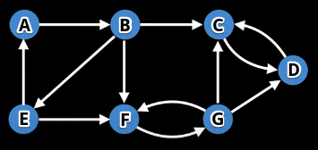
Algorithm output:

[[3, 2], [6, 5], [4, 1, 0]] # actual output
[[D, C], [G, F], [E, B, A]] # node lettering correspondence

Topological ordering:

DFS details:

""" 

(   A   B  C  D   E   F   G
  [ 1,  2, 3, 4,  7,  8,  9],   # discovered
  [14, 13, 6, 5, 12, 11, 10],   # finished
  [-1,  0, 1, 2,  1,  4,  5],   # predecessors
  {                             # edge classifications
    ('A', 'B'): 'treeEdge', 
    ('B', 'C'): 'treeEdge', 
    ('C', 'D'): 'treeEdge', 
    ('D', 'C'): 'backEdge', 
    ('B', 'E'): 'treeEdge', 
    ('E', 'A'): 'backEdge', 
    ('E', 'F'): 'treeEdge', 
    ('F', 'G'): 'treeEdge', 
    ('G', 'C'): 'crossEdge', 
    ('G', 'D'): 'crossEdge', 
    ('G', 'F'): 'backEdge', 
    ('B', 'F'): 'forwardEdge'
  }
)

"""

Working code:

Loading...

Output

Click "Run Code" to see the output here

Example 3

Graph visual (source):

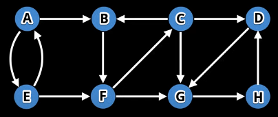
Algorithm output:

[[7, 6, 3], [2, 5, 1], [4, 0]] # actual output
[[H, G, D], [C, F, B], [E, A]] # node lettering correspondence

Topological ordering:

DFS details:

""" 

(
  [ 1,  2,  4,  5, 14,  3, 6, 7],   # discovered
  [16, 13, 11, 10, 15, 12, 9, 8],   # finished
  [-1,  0,  5,  2,  0,  1, 3, 6],   # predecessors
  {                                 # edge classifications
    ('A', 'B'): 'treeEdge', 
    ('B', 'F'): 'treeEdge', 
    ('F', 'C'): 'treeEdge', 
    ('C', 'B'): 'backEdge', 
    ('C', 'D'): 'treeEdge', 
    ('D', 'G'): 'treeEdge', 
    ('G', 'H'): 'treeEdge', 
    ('H', 'D'): 'backEdge', 
    ('C', 'G'): 'forwardEdge', 
    ('F', 'G'): 'forwardEdge', 
    ('A', 'E'): 'treeEdge', 
    ('E', 'A'): 'backEdge', 
    ('E', 'F'): 'crossEdge'
  }
)

"""

Working code:

Loading...

Output

Click "Run Code" to see the output here

Example 4

Graph visual (source):

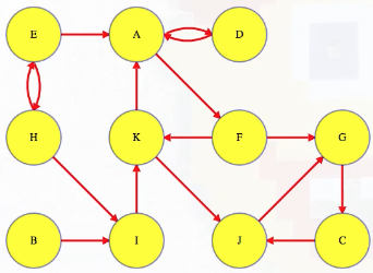
Algorithm output:

[[9, 2, 6], [10, 5, 3, 0], [8], [1], [7, 4]] # actual output
[[J, C, G], [ K, F, D, A], [I], [B], [H, E]] # node lettering correspondence

Topological ordering:

DFS details:

""" 

(   A   B  C  D   E   F   G   H   I  J   K
  [ 1, 15, 6, 2, 19,  4,  5, 20, 16, 7, 11],  # discovered
  [14, 18, 9, 3, 22, 13, 10, 21, 17, 8, 12],  # finished
  [-1, -1, 6, 0, -1,  0,  5,  4,  1, 2,  5],  # predecessors
  {                                           # edge classifications
    ('A', 'D'): 'treeEdge', 
    ('D', 'A'): 'backEdge', 
    ('A', 'F'): 'treeEdge', 
    ('F', 'G'): 'treeEdge', 
    ('G', 'C'): 'treeEdge', 
    ('C', 'J'): 'treeEdge', 
    ('J', 'G'): 'backEdge', 
    ('F', 'K'): 'treeEdge', 
    ('K', 'A'): 'backEdge', 
    ('K', 'J'): 'crossEdge', 
    ('B', 'I'): 'treeEdge', 
    ('I', 'K'): 'crossEdge', 
    ('E', 'A'): 'crossEdge', 
    ('E', 'H'): 'treeEdge', 
    ('H', 'E'): 'backEdge', 
    ('H', 'I'): 'crossEdge'
  }
)

"""

Working code:

Loading...

Output

Click "Run Code" to see the output here

Example 5

Graph visual (source):

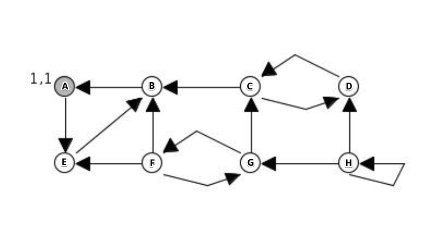
Algorithm output:

[[1, 4, 0], [3, 2], [6, 5], [7]] # actual output
[[B, E, A], [D, C], [G, F], [H]] # node lettering correspondence

Topological ordering:

DFS details:

""" 

(
  [ 1, 3,  7, 8, 2, 11, 12, 15],  # discovered
  [ 6, 4, 10, 9, 5, 14, 13, 16],  # finished
  [-1, 4, -1, 2, 0, -1,  5, -1],  # predecessors
  {                               # edge classifications
    ('A', 'E'): 'treeEdge', 
    ('E', 'B'): 'treeEdge', 
    ('B', 'A'): 'backEdge', 
    ('C', 'B'): 'crossEdge', 
    ('C', 'D'): 'treeEdge', 
    ('D', 'C'): 'backEdge', 
    ('F', 'B'): 'crossEdge', 
    ('F', 'E'): 'crossEdge', 
    ('F', 'G'): 'treeEdge', 
    ('G', 'C'): 'crossEdge', 
    ('G', 'F'): 'backEdge', 
    ('H', 'D'): 'crossEdge', 
    ('H', 'H'): 'backEdge'
  }
)

"""

Working code:

Loading...

Output

Click "Run Code" to see the output here

---